
Module maputils is your toolkit for writing small and dedicated applications for the inspection and of FITS headers, the extraction, manipulation display and re-projection of (FITS) data, interactive inspection of this data (color editing) and for the creation of plots with world coordinate information. Many of the examples in this tutorial are small applications which can be used with your own data with only small modifications (like file names etc.).
Module maputils provides methods to draw a graticule in a plot showing the world coordinates in the given projection and sky system. One can plot spatial rulers which show offsets of constant distance whatever the projection of the map is. We will also demonstrate how to create a so called all-sky plot
The module combines the functionality in modules wcs and celestial from the Kapteyn package, together with Matplotlib, into a powerful module for the extraction and display of FITS image data or external data described by a FITS header or a Python dictionary with FITS keywords (so in principle you are not bound to FITS files).
We show examples of:
- overlays of different graticules (each representing a different sky system),
- plots of data slices from a data set with more than two axes (e.g. a FITS file with channel maps from a radio interferometer observation)
- plots with a spectral axis with a ‘spectral translation’ (e.g. Frequency to Radio velocity)
- rulers showing offsets in spatial distance
- overlay a second image on a base image
- plot that covers the entire sky (allsky plot)
- mosaics of multiple images (e.g. HI channel maps)
- a simple movie loop program to view ‘channel’ maps.
We describe simple methods to add interaction to the Matplotlib canvas e.g. for changing color maps or color ranges.
In this tutorial we assume a basic knowledge of FITS files. Also a basic knowledge of Matplotlib is handy but not necessary to be able to modify the examples in this tutorial to suit your own needs. For useful references see information below.
See also
Building small display- and analysis utilities with maputils is easy. The complexity is usually in finding the right parameters in the right methods or functions to achieve special effects. The structure of a script to create a plot using maputils can be summarized with:
- Import maputils module
- Get data from a FITS file or another source
- Create a plot window and tell it where to plot your data
- From the object that contains your data, derive new objects
- With the methods of these new objects, plot an image, contours, graticule etc.
- Do the actual plotting and in a second step fine tune plot properties of various objects
- Inspect, print or save your plot or save your new data to file on disk.
In the example below it is easy to identify these steps:
Example: mu_basic1.py - Show image and allow for color interaction
1 2 3 4 5 6 7 8 9 10 11 12 | from kapteyn import maputils
from matplotlib import pyplot as plt
f = maputils.FITSimage("m101.fits")
fig = plt.figure()
frame = fig.add_subplot(1,1,1)
annim = f.Annotatedimage(frame)
annim.Image()
annim.Graticule()
annim.plot()
annim.interact_imagecolors()
plt.show()
|
With module maputils one can extract image data from a FITS file, modify it and write it to another FITS file on disk. The methods we use for these purposes are based on package PyFITS (or the equivalent in Astropy, astropy.io.fits) but are adapted to function in the environment of the Kapteyn Package. Note that PyFITS is not part of the Kapteyn Package.
With maputils one can also extract data slices from data described by more than two axes (e.g. images as function of velocity or polarization). For data with only two axes, it can swap those axes (e.g. to swap R.A. and Declination). Also the limits of the data can be set to extract part of 2-dimensional data. To be able to create plots of unfamiliar data without any user interaction, you need to know some of the characteristics of this data before you can extract the right slice. Module maputils provides routines that can display this relevant information.
First you need to create an object from class maputils.FITSimage. Some information is extracted from the FITS header directly. Other information is extracted from attributes of a wcs.Projection object defined in module wcs. Method maputils.FITSimage.str_axisinfo() gets its information from a header and its associated Projection object. It provides information about things like the sky system and the spectral system, as strings, so the method is suitable to get verbose information for display on terminals and in gui’s.
Next we show a simple script which prints meta information of the FITS file ngc6946.fits:
Example: mu_fitsutils.py - Print meta data from FITS header or Python dictionary
1 2 3 4 5 6 7 8 9 10 11 12 13 14 15 16 17 18 19 20 21 22 23 | from kapteyn import maputils
from matplotlib import pylab as plt
fitsobject = maputils.FITSimage('ngc6946.fits')
print("HEADER:\n")
print fitsobject.str_header()
print("\nAXES INFO:\n")
print fitsobject.str_axisinfo()
print("\nEXTENDED AXES INFO:\n")
print fitsobject.str_axisinfo(long=True)
print("\nAXES INFO for image axes only:\n")
print fitsobject.str_axisinfo(axnum=fitsobject.axperm)
print("\nAXES INFO for non existing axis:\n")
print fitsobject.str_axisinfo(axnum=4)
print("SPECTRAL INFO:\n")
fitsobject.set_imageaxes(axnr1=1, axnr2=3)
print fitsobject.str_spectrans()
|
This code generates the following output:
1 2 3 4 5 6 7 8 9 10 11 12 13 14 15 16 17 18 19 20 21 22 23 24 25 26 27 28 29 30 31 32 33 34 35 36 37 38 39 40 41 | print """
HEADER:
SIMPLE = T / SIMPLE FITS FORMAT
BITPIX = -32 / NUMBER OF BITS PER PIXEL
NAXIS = 3 / NUMBER OF AXES
NAXIS1 = 100 / LENGTH OF AXIS
etc.
AXES INFO:
Axis 1: RA---NCP from pixel 1 to 100
{crpix=51 crval=-51.2821 cdelt=-0.007166 (DEGREE)}
{wcs type=longitude, wcs unit=deg}
etc.
EXTENDED AXES INFO:
axisnr - Axis number: 1
axlen - Length of axis in pixels (NAXIS): 100
ctype - Type of axis (CTYPE): RA---NCP
axnamelong - Long axis name: RA---NCP
axname - Short axis name: RA
etc.
WCS INFO:
Current sky system: Equatorial
reference system: ICRS
Output sky system: Equatorial
Output reference system: ICRS
etc.
SPECTRAL INFO:
0 FREQ-V2F (Hz)
1 ENER-V2F (J)
2 WAVN-V2F (1/m)
3 VOPT-V2W (m/s)
etc.
"""
|
The example extracts data from a FITS file on disk as given in the example code. To make the script a real utility one should allow the user to enter a file name. This can be done with Python’s raw-input function but to make it robust one should check the existence of a file, and if a FITS file has more than one header, one should prompt the user to specify the header. We also have to deal with alternate headers for world coordinate systems (WCS) etc. etc.
Note
To facilitate parameter settings we implemented so called prompt function. These are external functions which read context in a terminal and then set reasonable defaults for the required parameters in a prompt. These functions can serve as templates for more advanced functions which are used in gui environments.
The projection class from wcs interprests and stores the header information. It serves as the interface between maputils and the library WCSLIB.
Example: mu_projection.py - Get data from attributes of the projection system
1 2 3 4 5 6 7 8 9 10 11 12 13 | from kapteyn import maputils
print "Projection object from FITSimage:"
fitsobj = maputils.FITSimage("mclean.fits")
print "crvals:", fitsobj.convproj.crval
fitsobj.set_imageaxes(1,3)
print "crvals after axes specification:", fitsobj.convproj.crval
fitsobj.set_spectrans("VOPT-???")
print "crvals after setting spectral translation:", fitsobj.convproj.crval
print "Projection object from Annotatedimage:"
annim = fitsobj.Annotatedimage()
print "crvals:", annim.projection.crval
|
The output:
Projection object from FITSimage:
crvals: (178.7792, 53.655000000000001)
crvals after axes specification: (178.7792, 1415418199.4170001, 53.655000000000001)
crvals after setting spectral translation: (178.7792, 1050000.0000000042, 53.655000000000001)
Projection object from Annotatedimage:
crvals: (178.7792, 1050000.0000000042, 53.655000000000001)
Explanation:
As soon as the FITSimage object is created, it is assumed that the first two axes are the axes of the data you want to display. After setting alternative axes, a slice is taken and the projection system is changed. Now it shows attributes in the order of the slice and we see a third value in the tuple with term:CRVAL‘s. That’s because the last value represents the necessary matching spatial axis which is needed to do conversions between pixels and world coordinates.
As a next step we set a spectral translation for the second axis which is a frequency axis. Again the projection system changes. We did set the translation to an optical velocity and the printed CRVAL is indeed the reference optical velocity from the header of this FITS file (1050 km/s).
When an object from class maputils.Annotatedimage is created, the projection data is copied from the maputils.FITSimage object. It can be accessed through the maputils.Annotatedimage.projection attribute (last line of the above example).
Class maputils.FITSimage extracts data from a FITS file so that a map can be plotted with its associated world coordinate system. So we have to specify a number of parameters to get the required image data. This is done with the following methods:
Header - The constructor maputils.FITSimage needs name and path of the FITS file. It can be a file on disk or an URL. The file can be zipped. A FITS file can contain more than one header data unit. If this is an issue you need to enter the number of the unit that you want to use. A case insensitive name of the hdu is also allowed. A FITS header can also contain one or more alternate headers. Usually these describe another sky or spectral system. We list three examples. The first is a complete description of the FITS header. The second get its parameters from an external ‘prompt’ function (see next section) and the third uses a prompt function with a pre specfication of parameter alter which sets the alternate header.
>>> fitsobject = maputils.FITSimage('alt2.fits', hdunr=0, alter='A', memmap=1)
>>> fitsobject = maputils.FITSimage(promptfie=maputils.prompt_fitsfile)
>>> fitsobject = maputils.FITSimage(promptfie=maputils.prompt_fitsfile, alter='A')
>>> fitsobject = maputils.FITSimage('NICMOSn4hk12010_mos.fits', hdunr='err')
Later we will also discuss examples where we use external headers (i.e. not from a FITS file, but as a Python dictionary) and external data (i.e. from another source or from processed data). The user/programmer is responsible for the right shape of the data. Here is a small example of processed data:
>>> f = maputils.FITSimage("m101.fits", externaldata=log(abs(fftA)+1.0))Axis numbers - Method maputils.FITSimage.set_imageaxes() sets the axis numbers. These numbers follow the FITS standard, i.e. they start with 1. If the data has only two axes then it is possible to swap the axes. This method can be used in combination with an external prompt function. If the data has more than two axes, then the default value for the axis numbers axnr1=1 and axnr2=2. One can also enter the names of the axes. The input is case insensitive and a minimal match is applied to the axis names found in the CTYPE keywords in the header. Examples are:
>>> fitsobject.set_imageaxes(promptfie=maputils.prompt_imageaxes)
>>> fitsobject.set_imageaxes(axnr1=2, axnr2=1)
>>> fitsobject.set_imageaxes(2,1)         # swap
>>> fitsobject.set_imageaxes(1,3)         # XV map
>>> fitsobject.set_imageaxes('R','D')     # RA-DEC map
>>> fitsobject.set_imageaxes('ra','freq') # RA-FREQ map
Data slices from data sets with more than two axes - For an artificial set called ‘manyaxes.fits’, we want to extract one spatial map. The axes order is [frequency, declination, right ascension, stokes]. We extract a data slice at FREQ=2 and STOKES=1. This spatial map is obtained with the following lines:
>>> fitsobject = maputils.FITSimage('manyaxes.fits') # FREQ-DEC-RA-STOKES
>>> fitsobject.set_imageaxes(axnr1=3, axnr2=2, slicepos=(2,1))
Coordinate limits - If you want to extract only a part of the image then you need to set limits for the pixel coordinates. This is set with maputils.FITSimage.set_limits(). The limits can be set manually or with a prompt function. Here are examples of both:
>>> fitsobject.set_limits(pxlim=(20,40), pylim=(22,38))
>>> fitsobject.set_limits((20,40), (22,38))
>>> fitsobject.set_limits(promptfie=maputils.prompt_box)
Output sky definition - For conversions between pixel- and world coordinates one can define to which output sky definition the world coordinates are related. The sky parameters are set with maputils.FITSimage.set_skyout(). The syntax for a sky definition (sky system, reference system, equinox, epoch of observation) is documented in celestial.skymatrix().
>>> fitsobject = maputils.FITSimage('m101.fits')
>>> fitsobject.set_skyout("Equatorial, J1952, FK4_no_e, J1980")
    or:
>>> fitsobject.set_skyout(promptfie=maputils.prompt_skyout)
Writing data to a FITS file or to append data to a FITS file is also possible. The method written for these purposes is called writetofits(). It has parameters to scale data and it is possible to skip writing history and comment keywords. Have a look at the examples:
>>> # Write data with scaling
>>> fitsobject.writetofits(history=True, comment=True,
                           bitpix=fitsobject.bitpix,
                           bzero=fitsobject.bzero,
                           bscale=fitsobject.bscale,
                           blank=fitsobject.blank)
>>> # Append data to existing FITS file
>>> fitsobject.writetofits("standard.fits", append=True, history=False, comment=False)
Usually one doesn’t know exactly what’s in the header of a FITS file or one has limited knowledge about the input parameters in maputils.FITSimage.set_imageaxes() Then a helper function to get the right input is available. It is called maputils.prompt_imageaxes() which works only in a terminal.
But a complete description of the world coordinate system implies also that it should possible to set limits for the pixel coordinates (e.g. to extract the most interesting part of the entire image) and specify the sky system in which we present a spatial map or the spectral translation (e.g. from frequency to velocity) for an image with a spectral axis. It is easy to turn our basic script into an interactive application that sets all necessary parameters to extract the required image data from a FITS file. The next script is an example how we use prompt functions to ask a user to enter relevant information. These prompt functions are external functions. They are aware of the data context and set reasonable defaults for the required parameters.
Example: mu_getfitsimage.py - Use prompt functions to set attributes of the FITSimage object and print information about the world coordinate system
1 2 3 4 5 6 7 8 9 10 11 12 | from kapteyn import maputils
fitsobject = maputils.FITSimage(promptfie=maputils.prompt_fitsfile)
print fitsobject.str_axisinfo()
fitsobject.set_imageaxes(promptfie=maputils.prompt_imageaxes)
fitsobject.set_limits(promptfie=maputils.prompt_box)
print fitsobject.str_spectrans()
fitsobject.set_spectrans(promptfie=maputils.prompt_spectrans)
fitsobject.set_skyout(promptfie=maputils.prompt_skyout)
print("\nWCS INFO:")
print fitsobject.str_wcsinfo()
|
Example: fitsview - Use prompt functions to create a script that displays a FITS image
As a summary we present a small but handy utility to display a FITS image using prompt functions. The name of the FITS file can be a command line argument e.g.: ./fitsimage m101.fits For this you need to download the code and make the script executable (e.g. chmod u+x) and run it from the command line like:
>>> ./fitsview m101.fits
1 2 3 4 5 6 7 8 9 10 11 12 13 14 15 16 17 18 19 20 21 22 23 24 25 26 27 28 29 30 31 32 33 34 35 36 | #!/usr/bin/env python
from kapteyn import wcsgrat, maputils
from matplotlib import pylab as plt
import sys
# Create a maputils FITS object from a FITS file on disk
if len(sys.argv) > 1:
filename = sys.argv[1]
fitsobject = maputils.FITSimage(filespec=filename,
promptfie=maputils.prompt_fitsfile, prompt=False)
else:
fitsobject = maputils.FITSimage(promptfie=maputils.prompt_fitsfile)
fitsobject.set_imageaxes(promptfie=maputils.prompt_imageaxes)
fitsobject.set_limits(promptfie=maputils.prompt_box)
fitsobject.set_skyout(promptfie=maputils.prompt_skyout)
fitsobject.set_spectrans(promptfie=maputils.prompt_spectrans)
clipmin, clipmax = maputils.prompt_dataminmax(fitsobject)
# Get connected to Matplotlib
fig = plt.figure()
frame = fig.add_subplot(1,1,1)
# Create an image to be used in Matplotlib
annim = fitsobject.Annotatedimage(frame, clipmin=clipmin, clipmax=clipmax)
annim.Image()
annim.Graticule()
#annim.Contours()
frame.set_title(fitsobject.filename, y=1.03)
annim.plot()
annim.interact_toolbarinfo()
annim.interact_imagecolors()
annim.interact_writepos()
plt.show()
|
If one is interested in displaying image data only (i.e. without any wcs information) then we need very few lines of code as we show in the next example.
Example: mu_simple.py - Minimal script to display image data
from kapteyn import maputils
from matplotlib import pyplot as plt

f = maputils.FITSimage("m101.fits")
mplim = f.Annotatedimage()
im = mplim.Image()
mplim.plot()

plt.show()
(Source code, png, hires.png, pdf)

Explanation:
This is a simple script that displays an image using the defaults for the axes, the limits, the color map and many other properties. From an object from class maputils.FITSimage an object from class maputils.FITSimage.Annotatedimage is derived.
This object has methods to create other objects (image, contours, graticule, ruler etc.) that can be plotted with Matplotlib. To plot these objects we need to call method maputils.Annotatedimage.plot()
If you are only interested in displaying the image and don’t want any white space around the plot then you need to specify a Matplotlib frame as parameter for maputils.Annotatedimage(). This frame is created with Matplotlib’s add_subplot() or add_axes(). The latter has options to specify origin and size of the frame in so called normalized coordinates [0,1]. Note that images are displayed while preserving the pixel aspect ratio. Therefore images are scaled to fit either the given width or the given height.
In the next example we reduce whitespace and use keyword parameters cmap, clipmin and clipmax to set a color map and the clip levels between which the color mapping is applied.
Example: mu_withimage.py - Display image data using keyword parameters
1 2 3 4 5 6 7 8 9 10 11 12 13 14 15 | from kapteyn import maputils
from matplotlib import pyplot as plt
fitsobj = maputils.FITSimage("m101.fits")
fitsobj.set_limits((180,344), (180,344))
fig = plt.figure(figsize=(4,4))
frame = fig.add_axes([0,0,1,1])
annim = fitsobj.Annotatedimage(frame, cmap="spectral", clipmin=10000, clipmax=15500)
annim.Image(interpolation='spline36')
print "clip min, max:", annim.clipmin, annim.clipmax
annim.plot()
plt.show()
|
(Source code, png, hires.png, pdf)

Fig.: mu_withimage.py - Image with non default plot frame and parameters for color map and clip levels.
It is possible to compose an image from three separate images which represent a red, green and blue component. In this case you need to create an maputils.Annotatedimage object first. The data associated with this image can be used to draw e.g. contours, while the parameters of the method maputils.Annotatedimage.RGBimage() compose the RGB image. The maputils.Annotatedimage.RGBimage() method creates a new data array and inserts your R, G & B images in the right place. Then it scales the composed data to a range between 0 and 1. For an RGB image we don’t apply interactive color bar editing, but allow for the use of a function or lambda expression to rescale the data to enhance features. In the example we used keyword parameter fun to square the data to enhance the image a bit.
Example: mu_rgbdemo.py - display RGB image
1 2 3 4 5 6 7 8 9 10 11 12 13 14 15 16 17 18 19 20 21 22 23 24 25 26 27 28 29 30 31 32 33 34 35 | from kapteyn import maputils
from matplotlib import pyplot as plt
# In the comments we show how to set a smaller box t display
f_red = maputils.FITSimage('m101_red.fits')
#f_red.set_limits((200,300),(200,300))
f_green = maputils.FITSimage('m101_green.fits')
#f_green.set_limits((200,300),(200,300))
f_blue = maputils.FITSimage('m101_blue.fits')
#f_blue.set_limits((200,300),(200,300))
# Show the three components R,G & B separately
# Show Z values when moving the mouse
fig = plt.figure()
frame = fig.add_subplot(2,2,1); frame.set_title("Red with noise")
a = f_red.Annotatedimage(frame); a.Image()
a.interact_toolbarinfo(wcsfmt=None, zfmt="%g")
frame = fig.add_subplot(2,2,2); frame.set_title("Greens are 1")
a = f_green.Annotatedimage(frame); a.Image()
a.interact_toolbarinfo(wcsfmt=None, zfmt="%g")
frame = fig.add_subplot(2,2,3); frame.set_title("Blues are 1")
a = f_blue.Annotatedimage(frame); a.Image()
a.interact_toolbarinfo(wcsfmt=None, zfmt="%g")
# Plot the composed RGB image
frame = fig.add_subplot(2,2,4); frame.set_title("RGB composed of previous")
annim = f_red.Annotatedimage(frame)
annim.RGBimage(f_red, f_green, f_blue, fun=lambda x:x*x, alpha=1)
# Note: color interaction not possible (RGB is fixed)
annim.interact_toolbarinfo(wcsfmt=None, zfmt="%g")
# Write RGB values to terminal after clicking left mouse button
annim.interact_writepos(pixfmt=None, wcsfmt="%.12f", zfmt="%.3e", hmsdms=False)
maputils.showall()
|
(Source code, png, hires.png, pdf)

Explanation:
Three FITS files contain data in rectangular shapes in different positions. If you want to use only a part of the images you need to set limits (with method set_limits()) for each image separately. The shapes in these example data files have values 1 (or near 1) and do overlap to illustrate the composition of a new color. The region where three shapes overlap is white in the composed output image. For each RGB component a maputils.FITSimage is created. One of these is used to make a maputils.FITSimage.Annotatedimage object. The three FITSimage objects are used as parameters for method maputils.Annotatedimage.RGBimage() to set the individual components of a RGB image. The red component is a bit special because we added some Gaussian noise to it. A second parameter used in the method is alpha. This is an alpha factor which applies to all the pixels in the composed map.
This script also displays a message in the message tool bar with information about mouse positions and the corresponding image value. For an RGB image, all three image values (z values) are displayed. The format of the message is changed with parameters in maputils.Annotatedimage.interact_toolbarinfo() as in:
>>> annim.interact_toolbarinfo(wcsfmt=None, zfmt="%g")
In the previous example we specified a size in inches for the figure. We provide a method maputils.FITSimage.get_figsize() to set the figure size in cm. Enter only the direction for which you want to set the size. The other size is calculated using the pixel aspect ratio, but then it is not garanteed that all labels will fit. The method is used as follows:
>>> fig = plt.figure(figsize=f.get_figsize(xsize=15, cm=True))
Module maputils can create graticule objects with method maputils.Annotatedimage.Graticule(). But in fact the method that does all the work is defined in module wcsgrat So in the next sections we often refer to module wcsgrat.
Module wcsgrat creates a graticule for a given header with WCS information. That implies that it finds positions on a curve in 2 dimensions in image data for which one of the world coordinates is a constant value. These positions are stored in a graticule object. The positions at which these lines cross one of the sides of the rectangle (made up by the limits in pixels in both x- and y-direction), are stored in a list together with a text label showing the world coordinate of the crossing.
Example: mu_axnumdemosimple.py - Simple plot using defaults
from kapteyn import maputils
from matplotlib import pyplot as plt

fitsobj = maputils.FITSimage("m101.fits")
mplim = fitsobj.Annotatedimage()
graticule = mplim.Graticule()
mplim.plot()

plt.show()
(Source code, png, hires.png, pdf)
Explanation:
The script opens an existing FITS file. Its header is parsed by methods in module wcs and methods from classes in module wcsgrat calculate the graticule data. A plot is made with Matplotlib. Note the small rotation of the graticules.
The recipe:
- Given a FITS file on disk (m101.fits) we want to plot a graticule for the spatial axes in the FITS file.
- The necessary information is retrieved from the FITS header with PyFITS through class maputils.FITSimage.
- To plot something we need to tell method maputils.FITSimage.Annotatedimage() in which frame it must plot. Therefore we need a Matplotlib figure instance and a Matplotlib Axes instance (which we call a frame in the context of maputils).
- A graticule representation is calculated by maputils.Annotatedimage.Graticule() and stored in object grat. The maximum number of defaults are used.
- Finally we tell the Annotated image object mplim to plot itself and display the result with Matplotlib’s function show(). This last step can be compressed to one statement: maputils.showall() which plots all the annotated images in your script at once and then call Matplotlib’s function show().
The wcsgrat module estimates the ranges in world coordinates in the coordinate system defined in your FITS file. The method is just brute force. This is the only way to get good estimates for large maps, rotated maps maps with weird projections (e.g. Bonne) etc. It is also possible to enter your own world coordinates to set limits. Methods in this module calculate ‘nice’ numbers to annotate the plot axes and to set default plot attributes.
Hint: Matplotlib versions older than 0.98 use module pylab instead of pyplot. You need to change the import statement to: from matplotlib import pylab as plt
Probably you already have many questions about what wcsgrat can do more:
- Is it possible to draw labels only and no graticule lines?
- Can I change the starting point and step size for the coordinate labels?
- Is it possible to change the default tick label format?
- Can I change the default titles along the axes?
- Is it possible to highlight (e.g. by changing color) just one graticule line?
- Can I plot graticules in maps with one spatial- and one spectral coordinate?
- Can I control the aspect ratio of the plot?
- Is it possible to set limits on pixel coordinates?
In the following sections we will give a number of examples to answer most of these questions.
For data sets with more than 2 axes or data sets with swapped axes (e.g. Declination as first axis and Right Ascension as second), we need to make a choice of the axes and axes order. To demonstrate this we created a FITS file with four axes. The order of the axes is uncommon and should only demonstrate the flexibility of the maputils module. We list the data for these axes in this ‘artificial’ FITS file:
Filename: manyaxes.fits
No.    Name         Type      Cards   Dimensions   Format
0    PRIMARY     PrimaryHDU      44  (10, 50, 50, 4)  int32
Axis  1 is FREQ   runs from pixel 1 to    10  (crpix=5 crval,cdelt=1.37835, 9.76563e-05 GHZ)
Axis  2 is DEC    runs from pixel 1 to    50  (crpix=30 crval,cdelt=45, -0.01 DEGREE)
Axis  3 is RA     runs from pixel 1 to    50  (crpix=25 crval,cdelt=30, -0.01 DEGREE)
Axis  4 is POL    runs from pixel 1 to     4  (crpix=1 crval,cdelt=1000, 10 STOKES)
You can download the file manyaxes.fits for testing. The world coordinate system is arbitrary.
Example: mu_manyaxes.py - Selecting WCS axes from a FITS file with NAXIS > 2
1 2 3 4 5 6 7 8 9 10 11 12 13 14 15 16 17 18 19 20 21 22 23 24 25 26 27 28 29 30 31 32 33 34 35 36 37 38 39 40 41 42 43 44 45 46 47 48 49 50 51 52 53 54 55 56 57 58 59 60 61 | from kapteyn import maputils
from matplotlib import pyplot as plt
# 1. Read the header
fitsobj = maputils.FITSimage("manyaxes.fits")
# 2. Create a Matplotlib Figure and Axes instance
figsize=fitsobj.get_figsize(ysize=12, xsize=11, cm=True)
fig = plt.figure(figsize=figsize)
frame = fig.add_subplot(1,1,1)
# 3. Create a graticule
fitsobj.set_imageaxes('freq','pol')
mplim = fitsobj.Annotatedimage(frame)
grat = mplim.Graticule(starty=1000, deltay=10)
# 4. Show the calculated world coordinates along y-axis
print "The world coordinates along the y-axis:", grat.ystarts
# 5. Show header information in attributes of the Projection object
# The projection object of a graticule is attribute 'gmap'
print "CRVAL, CDELT from header:", grat.gmap.crval, grat.gmap.cdelt
# 6. Set a number of properties of the graticules and plot axes
grat.setp_tick(plotaxis="bottom",
fun=lambda x: x/1.0e9, fmt="%.4f",
rotation=-30 )
grat.setp_axislabel("bottom", label="Frequency (GHz)")
grat.setp_gratline(wcsaxis=0, position=grat.gmap.crval[0],
tol=0.5*grat.gmap.cdelt[0], color='r')
grat.setp_ticklabel(plotaxis="left", position=1000, color='m', fmt="I")
grat.setp_ticklabel(plotaxis="left", position=1010, color='b', fmt="Q")
grat.setp_ticklabel(plotaxis="left", position=1020, color='r', fmt="U")
grat.setp_ticklabel(plotaxis="left", position=1030, color='g', fmt="V")
grat.setp_axislabel("left", label="Stokes parameters")
# 7. Set a title for this frame
title = r"""Polarization as function of frequency at:
$(\alpha_0,\delta_0) = (121^o,53^o)$"""
t = frame.set_title(title, color='#006400', y=1.01, linespacing=1.4)
# 8. Add labels inside plot
inlabs = grat.Insidelabels(wcsaxis=0, constval=1015,
deltapx=-0.15, rotation=90,
fontsize=10, color='r',
fun=lambda x: x*1e-9, fmt="%.4f.10^9")
w = grat.gmap.crval[0] + 0.2*grat.gmap.cdelt[0]
cv = grat.gmap.crval[1]
# Print without any formatting
inlab2 = grat.Insidelabels(wcsaxis=0, world=w, constval=cv,
deltapy=0.1, rotation=20,
fontsize=10, color='c')
pixel = grat.gmap.topixel((w,grat.gmap.crval[1]))
frame.plot( (pixel[0],), (pixel[1],), 'o', color='red' )
# 9. Plot the objects
maputils.showall()
|
(Source code, png, hires.png, pdf)

The plot shows a system of grid lines that correspond to non spatial axes and it will be no surprise that the graticule is a rectangular system. The example follows the same recipe as the previous ones and it shows how one selects the required plot axes in a FITS file. The axes are set with maputils.FITSimage.set_imageaxes() with two numbers. The first axis of a set is axis 1, the second 2, etc. (i.e. FITS standard). The default is (1,2) i.e. the first two axes in a FITS header.
For a R.A.-Dec. graticule one should enter for this FITS file:
>>> f.set_imageaxes(3,2)
Note
If a FITS file has data which has more than two dimensions or it has two dimensions but you want to swap the x- and y axis then you need to specify the relevant FITS axes with maputils.FITSimage.set_imageaxes(). The (FITS) axes numbers correspond to the number n in the FITS keyword CTYPEn (e.g. CTYPE3=’FREQ’ then the frequency axis corresponds to number 3).
Let’s study the plot in more detail:
The header shows a Stokes axes with an uncommon value for CRVAL and CDELT. We want to label four graticule lines with the familiar Stokes parameters. With the knowledge we have about this CRVAL and CDELT we tell the Graticule constructor to create 4 graticule lines (starty=1000, deltay=10).
The four positions are stored in attribute ystarts as in grat.ystarts. We use these numbers to change the coordinate labels into Stokes parameters with method wcsgrat.Graticule.setp_ticklabel()
>>> grat.setp_ticklabel(plotaxis="left", position=1000, color='m', fmt="I")We use wcsgrat.Insidelabels() to add coordinate labels inside the plot. We mark a position near CRVAL and plot a label and with the same method we added a single label at that position.
This example shows an important feature of the underlying module wcsgrat and that is its possibility to change properties of graticules, ticks and labels. We summarize:
- Graticule line properties are set with wcsgrat.Graticule.setp_gratline() or the equivalent wcsgrat.Graticule.setp_lineswcs1() or wcsgrat.Graticule.setp_lineswcs1(). The properties are all Matplotlib properties given as keyword arguments. One can apply these to all graticule lines, to one of the wcs types or to one graticule line (identified by its position in world coordinates).
- Graticule ticks (the intersections with the borders) are modified by method wcsgrat.Graticule.setp_tick(). Ticks are identified by either the wcs axis (e.g. longitude or latitude) or by one of the four rectangular plot axes or by a position in world coordinates. Combinations of these are also possible. Plot properties are given as Matplotlib keyword arguments. The labels can be scaled and formatted with parameters fun and fmt. Usually one uses method wcsgrat.Graticule.setp_ticklabel() to change tick labels and wcsgrat.Graticule.setp_tickmark() to change the tick markers.
- Ticks can be native to a plot axis (e.g. an pixel X axis which corresponds to a R.A. axis in world coordinates. But sometimes you can have ticks from two world coordinate axes along the same pixel axis (e.g. for a rotated plot). Then it is possible to control which ticks are plotted and which not. A tick mode for one or more plot/pixel axes is set with wcsgrat.Graticule.set_tickmode().
- The titles along one of the rectangular plot axes can be modified with wcsgrat.Graticule.setp_axislabel() which is a specialization of method wcsgrat.Graticule.setp_plotaxis(). A label text is set with parameter label and the plot properties are given as Matplotlib keyword arguments.
- Properties of labels inside a plot are set in the constructor wcsgrat.Insidelabels.setp_label().
- Properties of labels along a ruler are set with method rulers.Ruler.setp_label(). Properties of the ruler line can be changed with rulers.Ruler.setp_line()
- For labels along the plotaxes which correspond to pixel positions one can change the properties of the labels with maputils.Pixellabels.setp_label() while the properties of the markers can be changed with: maputils.Pixellabels.setp_marker()
Let’s summarize these methods in a table:
| Object | Properties method |
|---|---|
| Graticule line piece | wcsgrat.Graticule.setp_gratline() |
| Graticule tick marker | wcsgrat.Graticule.setp_tickmark() |
| Graticule tick_label | wcsgrat.Graticule.setp_ticklabel() |
| Axis label | wcsgrat.Graticule.setp_axislabel() |
| Inside label | wcsgrat.Insidelabels.setp_label() |
| Ruler labels | rulers.Ruler.setp_label() |
| Ruler line | rulers.Ruler.setp_line() |
| Pixel labels | maputils.Pixellabels.setp_label() |
| Pixel markers | maputils.Pixellabels.setp_marker() |
| Free graticule line | wcsgrat.Graticule.setp_linespecial() |
-Table- Objects related to graticules and their methods to set properties.
In the following sections we show some examples for changing the graticule properties. Note that for some methods we can identify objects either with the graticule line type (i.e. 0 or 1), the number or name of the plot axis ([0..4] or one of ‘left’, ‘bottom’, ‘right’, ‘top’ (or a minimal match of these strings). Some objects (e.g. tick labels) can also be identified by a position in world coordinates. Often also a combination of these identifiers can be used.
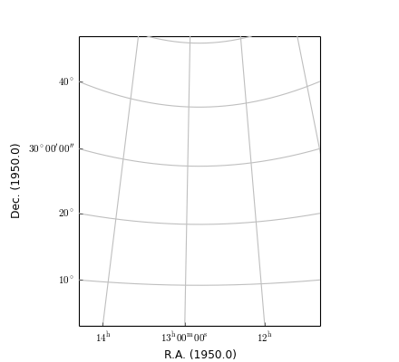
Example: mu_labeldemo.py - Properties of axis labels
1 2 3 4 5 6 7 8 9 10 11 12 13 14 15 16 17 18 19 20 21 22 23 24 25 26 27 28 29 30 31 32 33 34 35 36 37 | from kapteyn import maputils
from matplotlib import pylab as plt
header = {
'NAXIS': 2 ,
'NAXIS1': 100 ,
'NAXIS2': 100 ,
'CDELT1': -7.165998823000E-03 ,
'CRPIX1': 5.100000000000E+01 ,
'CRVAL1': -5.128208479590E+01 ,
'CTYPE1': 'RA---NCP ' ,
'CUNIT1': 'DEGREE ' ,
'CDELT2': 7.165998823000E-03 ,
'CRPIX2': 5.100000000000E+01 ,
'CRVAL2': 6.015388802060E+01 ,
'CTYPE2': 'DEC--NCP ' ,
'CUNIT2': 'DEGREE ' ,
}
fig = plt.figure(figsize=(6,5.2))
frame = fig.add_axes([0.15,0.15,0.8,0.8])
f = maputils.FITSimage(externalheader=header)
annim = f.Annotatedimage(frame)
grat = annim.Graticule()
grat.setp_axislabel(fontstyle='italic') # Apply to all
grat.setp_axislabel("top", visible=True, xpos=0.0, ypos=1.0, rotation=180)
grat.setp_axislabel("left",
backgroundcolor='y',
color='b',
style='oblique',
weight='bold',
ypos=0.3)
grat.setp_axislabel("bottom", # Label in LaTeX
label=r"$\mathrm{Right\ Ascension\ (2000)}$",
fontsize=14)
annim.plot()
plt.show()
|
(Source code, png, hires.png, pdf)

Example: mu_gratlinedemo.py - Properties of graticule lines
1 2 3 4 5 6 7 8 9 10 11 12 13 14 15 16 17 18 19 20 21 22 23 24 | from kapteyn import maputils
from matplotlib import pylab as plt
header = {'NAXIS': 2 ,'NAXIS1':100 , 'NAXIS2': 100 ,
'CDELT1': -7.165998823000E-03, 'CRPIX1': 5.100000000000E+01 ,
'CRVAL1': -5.128208479590E+01, 'CTYPE1': 'RA---NCP', 'CUNIT1': 'DEGREE ',
'CDELT2': 7.165998823000E-03 , 'CRPIX2': 5.100000000000E+01,
'CRVAL2': 6.015388802060E+01 , 'CTYPE2': 'DEC--NCP ', 'CUNIT2': 'DEGREE'
}
fig = plt.figure(figsize=(6,5.2))
frame = fig.add_subplot(1,1,1)
f = maputils.FITSimage(externalheader=header)
annim = f.Annotatedimage(frame)
grat = annim.Graticule()
grat.setp_gratline(lw=2)
grat.setp_gratline(wcsaxis=0, color='r')
grat.setp_gratline(wcsaxis=1, color='g')
grat.setp_gratline(wcsaxis=1, position=60.25, linestyle=':')
grat.setp_gratline(wcsaxis=0, position="20d34m0s", linestyle=':')
# If invisible, use: grat.setp_gratline(visible=False)
annim.plot()
plt.show()
|
(Source code, png, hires.png, pdf)

Note
If you don’t want to plot graticule lines, then use method wcsgrat.setp_gratline() with attribute visible set to False.
Example: mu_ticklabeldemo.py - Properties of graticule tick labels
1 2 3 4 5 6 7 8 9 10 11 12 13 14 15 16 17 18 19 20 21 22 23 24 25 26 27 28 29 30 | from kapteyn import maputils
from matplotlib import pylab as plt
header = {'NAXIS': 2 ,'NAXIS1':100 , 'NAXIS2': 100 ,
'CDELT1': -7.165998823000E-03, 'CRPIX1': 5.100000000000E+01 ,
'CRVAL1': -5.128208479590E+01, 'CTYPE1': 'RA---NCP', 'CUNIT1': 'DEGREE ',
'CDELT2': 7.165998823000E-03, 'CRPIX2': 5.100000000000E+01,
'CRVAL2': 6.015388802060E+01, 'CTYPE2': 'DEC--NCP ', 'CUNIT2': 'DEGREE'
}
fig = plt.figure()
frame = fig.add_axes([0.20,0.15,0.75,0.8])
f = maputils.FITSimage(externalheader=header)
annim = f.Annotatedimage(frame)
grat = annim.Graticule()
grat2 = annim.Graticule(skyout='Galactic')
grat.setp_ticklabel(plotaxis="bottom", position="20h34m", fmt="%g",
color='r', rotation=30)
grat.setp_ticklabel(plotaxis='left', color='b', rotation=20,
fontsize=14, fontweight='bold', style='italic')
grat.setp_ticklabel(plotaxis='left', color='m', position="60d0m0s",
fmt="DMS", tex=False)
grat.setp_axislabel(plotaxis='left', xpos=-0.25, ypos=0.5)
# Rotation is inherited from previous setting
grat2.setp_gratline(color='g')
grat2.setp_ticklabel(visible=False)
grat2.setp_axislabel(visible=False)
annim.plot()
plt.show()
|
(Source code, png, hires.png, pdf)

Example: mu_tickmarkerdemo.py - Properties of graticule tick markers
1 2 3 4 5 6 7 8 9 10 11 12 13 14 15 16 17 18 19 20 21 22 23 24 25 26 | from kapteyn import maputils
from matplotlib import pylab as plt
header = {'NAXIS': 2 ,'NAXIS1':100 , 'NAXIS2': 100 ,
'CDELT1': -7.165998823000E-03, 'CRPIX1': 5.100000000000E+01 ,
'CRVAL1': -5.128208479590E+01, 'CTYPE1': 'RA---NCP', 'CUNIT1': 'DEGREE ',
'CDELT2': 7.165998823000E-03 , 'CRPIX2': 5.100000000000E+01,
'CRVAL2': 6.015388802060E+01 , 'CTYPE2': 'DEC--NCP ', 'CUNIT2': 'DEGREE'
}
fig = plt.figure()
#frame = fig.add_axes([0.15,0.15,0.8,0.8])
frame = fig.add_subplot(1,1,1)
f = maputils.FITSimage(externalheader=header)
annim = f.Annotatedimage(frame)
grat = annim.Graticule()
grat.setp_gratline(visible=False)
grat.setp_ticklabel(plotaxis="bottom", position="20h34m", fmt="%6f")
grat.setp_tickmark(plotaxis="bottom", position="20h34m",
color='b', markeredgewidth=4, markersize=20)
fig.text(0.5, 0.5, "Empty", fontstyle='italic', fontsize=18, ha='center',
color='r')
annim.plot()
plt.show()
|
(Source code, png, hires.png, pdf)
Example: mu_tickmodedemo.py - Graticule’s tick mode
1 2 3 4 5 6 7 8 9 10 11 12 13 14 15 16 17 18 19 20 21 22 23 24 25 26 27 28 29 30 31 32 33 34 35 36 37 38 39 40 41 42 43 44 45 46 47 | from kapteyn import maputils
from matplotlib import pylab as plt
header = {'NAXIS': 2 ,'NAXIS1':100 , 'NAXIS2': 100 ,
'CDELT1': -7.165998823000E-03, 'CRPIX1': 5.100000000000E+01 ,
'CRVAL1': -5.128208479590E+01, 'CTYPE1': 'RA---NCP', 'CUNIT1': 'DEGREE ',
'CDELT2': 7.165998823000E-03 , 'CRPIX2': 5.100000000000E+01,
'CRVAL2': 6.015388802060E+01 , 'CTYPE2': 'DEC--NCP ', 'CUNIT2': 'DEGREE',
'CROTA2': 80
}
fig = plt.figure(figsize=(7,7))
fig.suptitle("Messy plot. Rotation is 80 deg.", fontsize=14, color='r')
fig.subplots_adjust(left=0.18, bottom=0.10, right=0.90,
top=0.90, wspace=0.95, hspace=0.20)
frame = fig.add_subplot(2,2,1)
f = maputils.FITSimage(externalheader=header)
annim = f.Annotatedimage(frame)
xpos = -0.42
ypos = 1.2
grat = annim.Graticule()
grat.setp_axislabel(plotaxis=0, xpos=xpos)
frame.set_title("Default", y=ypos)
frame2 = fig.add_subplot(2,2,2)
annim2 = f.Annotatedimage(frame2)
grat2 = annim2.Graticule()
grat2.setp_axislabel(plotaxis=0, xpos=xpos)
grat2.set_tickmode(mode="sw")
frame2.set_title("Switched ticks", y=ypos)
frame3 = fig.add_subplot(2,2,3)
annim3 = f.Annotatedimage(frame3)
grat3 = annim3.Graticule()
grat3.setp_axislabel(plotaxis=0, xpos=xpos)
grat3.set_tickmode(mode="na")
frame3.set_title("Only native ticks", y=ypos)
frame4 = fig.add_subplot(2,2,4)
annim4 = f.Annotatedimage(frame4)
grat4 = annim4.Graticule()
grat4.setp_axislabel(plotaxis=0, xpos=xpos)
grat4.set_tickmode(plotaxis=['bottom','left'], mode="Switch")
grat4.setp_ticklabel(plotaxis=['top','right'], visible=False)
frame4.set_title("Switched and cleaned", y=ypos)
maputils.showall()
|
(Source code, png, hires.png, pdf)

Example: mu_insidelabeldemo.py - Graticule ‘inside’ labels
1 2 3 4 5 6 7 8 9 10 11 12 13 14 15 16 17 18 19 20 21 22 23 24 25 26 27 | from kapteyn import maputils
from matplotlib import pylab as plt
header = {'NAXIS': 2 ,'NAXIS1':100 , 'NAXIS2': 100 ,
'CDELT1': -7.165998823000E-03, 'CRPIX1': 5.100000000000E+01 ,
'CRVAL1': -5.128208479590E+01, 'CTYPE1': 'RA---NCP', 'CUNIT1': 'DEGREE ',
'CDELT2': 7.165998823000E-03 , 'CRPIX2': 5.100000000000E+01,
'CRVAL2': 6.015388802060E+01 , 'CTYPE2': 'DEC--NCP ', 'CUNIT2': 'DEGREE'
}
fig = plt.figure()
frame = fig.add_axes([0.15,0.15,0.8,0.8])
f = maputils.FITSimage(externalheader=header)
annim = f.Annotatedimage(frame)
grat = annim.Graticule()
grat2 = annim.Graticule(skyout='Galactic')
grat2.setp_gratline(color='g')
grat2.setp_ticklabel(visible=False)
grat2.setp_axislabel(visible=False)
inswcs0 = grat2.Insidelabels(wcsaxis=0, deltapx=5, deltapy=5)
inswcs1 = grat2.Insidelabels(wcsaxis=1, constval='95d45m')
inswcs0.setp_label(color='r')
inswcs0.setp_label(position="96d0m", color='b', tex=False, fontstyle='italic')
inswcs1.setp_label(position="12d0m", fontsize=14, color='m')
annim.plot()
annim.interact_toolbarinfo()
plt.show()
|
(Source code, png, hires.png, pdf)

Example: mu_offsetaxes.py - Graticule offset labeling
1 2 3 4 5 6 7 8 9 10 11 12 13 14 15 16 17 18 19 20 21 22 23 24 25 26 27 28 29 30 31 32 33 34 35 36 37 38 39 40 41 42 43 44 45 46 47 48 49 50 51 52 53 54 55 56 57 58 59 60 | from kapteyn import maputils
from matplotlib import pylab as plt
def plotgrat(n, ax1, ax2, offsetx=None, offsety=None, unitsx=None):
f.set_imageaxes(ax1,ax2)
frame = fig.add_subplot(4,2,n)
annim = f.Annotatedimage(frame)
grat = annim.Graticule(offsetx=offsetx, offsety=offsety, unitsx=unitsx)
grat.setp_axislabel((0,1,2), fontsize=10)
grat.setp_ticklabel(fontsize=7)
xmax = annim.pxlim[1]+0.5; ymax = annim.pylim[1]+0.5
ruler = annim.Ruler(x1=xmax, y1=0.5, x2=xmax, y2=ymax,
lambda0=0.5, step=10.0,
units='arcmin',
fliplabelside=True)
ruler.setp_line(lw=2, color='r')
ruler.setp_label(clip_on=True, color='r', fontsize=9)
ruler2 = annim.Ruler(x1=0.5, y1=0.5, x2=xmax, y2=ymax,
lambda0=0.5, step=10.0/60.0,
fun=lambda x: x*60.0, fmt="%4.0f^\prime",
mscale=6, fliplabelside=True)
ruler2.setp_line(lw=2, color='b')
ruler2.setp_label(color='b', fontsize=9)
grat.setp_axislabel("right", label="Offset (Arcmin.)",
visible=True, backgroundcolor='y')
# Main ...
fig = plt.figure(figsize=(7,8))
fig.subplots_adjust(left=0.17, bottom=0.10, right=0.92,
top=0.93, wspace=0.24, hspace=0.34)
header = { 'NAXIS':3,'NAXIS1':100, 'NAXIS2':100 , 'NAXIS3':101 ,
#'CDELT1': -7.165998823000E-03,
'CDELT1': -11.165998823000E-03, 'CRPIX1': 5.100000000000E+01 ,
'CRVAL1': -5.128208479590E+01, 'CTYPE1': 'RA---NCP' , 'CUNIT1': 'DEGREE',
'CDELT2': 7.165998823000E-03, 'CRPIX2': 5.100000000000E+01,
'CRVAL2': 6.015388802060E+01, 'CTYPE2': 'DEC--NCP', 'CUNIT2': 'DEGREE',
'CDELT3': 4.199999809000E+00, 'CRPIX3': -2.000000000000E+01,
'CRVAL3': -2.430000000000E+02, 'CTYPE3': 'VELO-HEL', 'CUNIT3': 'km/s',
'EPOCH ': 2.000000000000E+03,
'FREQ0 ': 1.420405758370E+09
}
f = maputils.FITSimage(externalheader=header)
plotgrat(1,3,1)
plotgrat(2,1,3)
plotgrat(3,3,2)
plotgrat(4,2,3, unitsx="arcsec")
plotgrat(5,1,2, offsetx=True)
plotgrat(6,2,1)
plotgrat(7,3,1, offsetx=True, unitsx='km/s')
plotgrat(8,1,3, offsety=True)
maputils.showall()
|
(Source code, png, hires.png, pdf)

Example: mu_minorticks.py - Graticule with minor tick marks
1 2 3 4 5 6 7 8 9 10 11 12 13 14 15 16 17 18 19 20 21 22 23 24 25 26 27 28 29 30 31 32 | from kapteyn import maputils
from matplotlib import pyplot as plt
fitsobj = maputils.FITSimage("m101.fits")
fig = plt.figure()
fig.subplots_adjust(left=0.18, bottom=0.10, right=0.90,
top=0.90, wspace=0.95, hspace=0.20)
for i in range(4):
f = fig.add_subplot(2,2,i+1)
mplim = fitsobj.Annotatedimage(f)
if i == 0:
majorgrat = mplim.Graticule()
majorgrat.setp_gratline(visible=False)
elif i == 1:
majorgrat = mplim.Graticule(offsetx=True, unitsx='ARCMIN')
majorgrat.setp_gratline(visible=False)
elif i == 2:
majorgrat = mplim.Graticule(skyout='galactic', unitsx='ARCMIN')
majorgrat.setp_gratline(color='b')
else:
majorgrat = mplim.Graticule(skyout='galactic',
offsetx=True, unitsx='ARCMIN')
majorgrat.setp_gratline(color='b')
majorgrat.setp_tickmark(markersize=10)
majorgrat.setp_ticklabel(fontsize=6)
majorgrat.setp_plotaxis(plotaxis=[0,1], fontsize=10)
minorgrat = mplim.Minortickmarks(majorgrat, 3, 5,
color="#aa44dd", markersize=3, markeredgewidth=2)
maputils.showall()
plt.show()
|
(Source code, png, hires.png, pdf)

Explanation
Minor tick marks are created in the same way as major tick marks. They are created as a by-product of the instantiation of an object from class wcsgrat.Graticule. The method maputils.Annotatedimage.Minortickmarks() copies some properties of the major ticks graticule and then creates a new graticule object. The example shows 4 plots representing the same image in the sky.
- The default plot with minor tick marks
- Minor tick marks can also be applied on offset axes
- We selected another sky system for our graticule. The tick marks are now applied to the galactic coordinate system.
- This is the tricky plot. First of all we observe that the center of the offset axis is not in the middle of the bottom plot axis. This is because the Galactic sky system is plotted upon an equatorial system and therefore it is (at least for this part of the sky) rotated which causes the limits in world coordinates to be stretched. The start of the offset axis is calculated for the common limits in world coordinates and not just those along a plot axis. Secondly, one should observe that the graticule lines for the longitude follow the tick mark positions on the offset axis. And third, the offset seems to have different sign when compared to the Equatorial system. The reason for this is that we took a part of the sky where the Galactic system’s longitude runs in an opposite direction.
There are many options to control the labeling along each axis in a plot. There are options in the contructor of a Graticule object to give a start value (startx, starty, in grids or world coordinates) for the first label along an axis. This label is the label that is written with all relevant information. Other labels are derived from this one. If a step size is given (deltax or deltay) then this will be used as step between labels. A sequence of start values are used to plot labels at their corresponding positions (a value of the step size is overruled). Values for the label positions in startx, starty given as a string follow the rules described in positions. Step sizes, given as a string, can be appended by a unit.
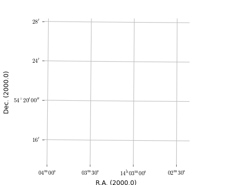
Example: mu_labelsspatial.py - Tricks to improve labeling of spatial axes
1 2 3 4 5 6 7 8 9 10 11 12 13 14 15 16 17 18 19 20 21 22 23 24 25 26 27 28 29 30 31 32 33 34 35 36 37 38 39 40 41 42 43 44 45 46 47 48 | from kapteyn import maputils
from matplotlib import pylab as plt
header = { 'NAXIS' : 3,
'BUNIT' : 'w.u.',
'CDELT1' : -1.200000000000E-03,
'CDELT2' : 1.497160000000E-03, 'CDELT3' : 97647.745732,
'CRPIX1' : 5, 'CRPIX2' : 6, 'CRPIX3' : 32,
'CRVAL1' : 1.787792000000E+02, 'CRVAL2' : 5.365500000000E+01,
'CRVAL3' : 1378471216.4292786,
'CTYPE1' : 'RA---NCP', 'CTYPE2' : 'DEC--NCP', 'CTYPE3' : 'FREQ-OHEL',
'CUNIT1' : 'DEGREE', 'CUNIT2' : 'DEGREE', 'CUNIT3' : 'HZ',
'DRVAL3' : 1.050000000000E+03,
'DUNIT3' : 'KM/S',
'FREQ0' : 1.420405752e+9,
'INSTRUME' : 'WSRT',
'NAXIS1' : 100, 'NAXIS2' : 100, 'NAXIS3' : 64
}
fig = plt.figure(figsize=(7,7))
fig.suptitle("Axis labels for spatial maps", fontsize=14, color='r')
fig.subplots_adjust(left=0.18, bottom=0.10, right=0.90,
top=0.90, wspace=0.95, hspace=0.20)
frame = fig.add_subplot(2,2,1)
f = maputils.FITSimage(externalheader=header)
f.set_imageaxes(1,2)
annim = f.Annotatedimage(frame)
# Default labeling
grat = annim.Graticule()
frame = fig.add_subplot(2,2,2)
annim = f.Annotatedimage(frame)
# Plot labels with start position and increment
grat = annim.Graticule(startx='11h55m', deltax="15 hmssec", deltay="3 arcmin")
frame = fig.add_subplot(2,2,3)
annim = f.Annotatedimage(frame)
# Plot labels in string only
grat = annim.Graticule(startx='11h55m 11h54m30s')
grat.setp_tick(plotaxis="bottom", texsexa=False)
frame = fig.add_subplot(2,2,4)
annim = f.Annotatedimage(frame)
grat = annim.Graticule(startx="178.75 deg", deltax="6 arcmin", unitsx="degree")
grat.setp_ticklabel(plotaxis="left", fmt="s")
maputils.showall()
|
(Source code, png, hires.png, pdf)
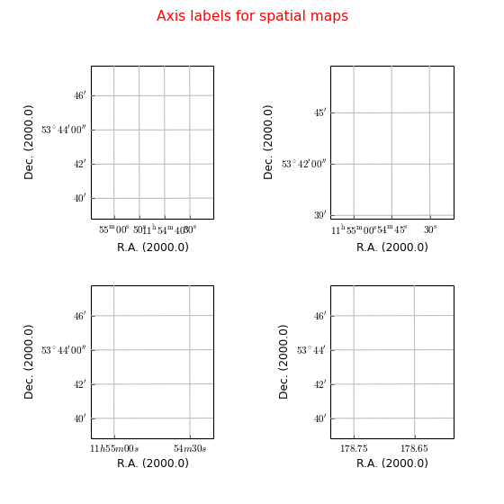
Explanation
Default
Plot labels with start position and increment. Note the use of a special unit ‘hmssec’. grat = annim.Graticule(startx='11h55m', deltax="15 hmssec", deltay="3 arcmin")
The LaTeX labeling is jumpy. Try it without superscripts (texsexa=False):
>>> grat = annim.Graticule(startx='11h55m 11h54m30s')
>>> grat.setp_tick(plotaxis="bottom", texsexa=False)
Force the y axis NOT to plot seconds. Force the x axis to plot in degrees.
>>> grat = annim.Graticule(startx="178.75 deg", deltax="6 arcmin", unitsx="degree")
>>> grat.setp_ticklabel(plotaxis="left", fmt="s")
More information about plotting in sexagesimal format is found in wcsgrat.makelabel()
Example: mu_labelsspectral.py - Tricks to improve labeling of spectral and offset axes
1 2 3 4 5 6 7 8 9 10 11 12 13 14 15 16 17 18 19 20 21 22 23 24 25 26 27 28 29 30 31 32 33 34 35 36 37 38 39 40 41 42 43 44 45 46 47 48 49 50 51 52 53 54 55 56 57 58 59 60 61 62 63 64 65 | from kapteyn import maputils
from matplotlib import pylab as plt
header = { 'NAXIS' : 3,
'BUNIT' : 'w.u.',
'CDELT1' : -1.200000000000E-03,
'CDELT2' : 1.497160000000E-03, 'CDELT3' : 97647.745732,
'CRPIX1' : 5, 'CRPIX2' : 6, 'CRPIX3' : 32,
'CRVAL1' : 1.787792000000E+02, 'CRVAL2' : 5.365500000000E+01,
'CRVAL3' : 1378471216.4292786,
'CTYPE1' : 'RA---NCP', 'CTYPE2' : 'DEC--NCP', 'CTYPE3' : 'FREQ-OHEL',
'CUNIT1' : 'DEGREE', 'CUNIT2' : 'DEGREE', 'CUNIT3' : 'HZ',
'DRVAL3' : 1.050000000000E+03,
'DUNIT3' : 'KM/S',
'FREQ0' : 1.420405752e+9,
'INSTRUME' : 'WSRT',
'NAXIS1' : 100, 'NAXIS2' : 100, 'NAXIS3' : 64
}
fig = plt.figure(figsize=(7,10))
fig.suptitle("Axis label tricks (spectral+spatial offset)", fontsize=14, color='r')
fig.subplots_adjust(left=0.18, bottom=0.10, right=0.90,
top=0.90, wspace=0.95, hspace=0.20)
frame = fig.add_subplot(3,2,1)
f = maputils.FITSimage(externalheader=header)
f.set_imageaxes(3,2, slicepos=1)
annim = f.Annotatedimage(frame)
# Default labeling
grat = annim.Graticule()
grat.setp_tick(plotaxis="bottom", rotation=90)
frame = fig.add_subplot(3,2,2)
annim = f.Annotatedimage(frame)
# Spectral axis with start and increment
grat = annim.Graticule(startx="1.378 Ghz", deltax="2 Mhz", starty="53d42m")
grat.setp_tick(plotaxis="bottom", fontsize=7, fmt='%.3f%+9e')
frame = fig.add_subplot(3,2,3)
annim = f.Annotatedimage(frame)
# Spectral axis with start and increment
grat = annim.Graticule(spectrans="WAVE", startx="21.74 cm",
deltax="0.04 cm", starty="0.5")
frame = fig.add_subplot(3,2,4)
annim = f.Annotatedimage(frame)
# Spectral axis with start and increment
grat = annim.Graticule(spectrans="VOPT", startx="9120 km/s",
deltax="400 km/s", unitsy="arcsec")
grat.setp_tick(plotaxis="bottom", fontsize=7)
frame = fig.add_subplot(3,2,5)
annim = f.Annotatedimage(frame)
# Spectral axis with start and increment and unit
grat = annim.Graticule(spectrans="VOPT", startx="9000 km/s",
deltax="400 km/s", unitsx="km/s")
frame = fig.add_subplot(3,2,6)
annim = f.Annotatedimage(frame)
# Spectral axis with start and increment and formatter function
grat = annim.Graticule(spectrans="VOPT", startx="9000 km/s", deltax="400 km/s")
grat.setp_tick(plotaxis="bottom", fmt='%g', fun=lambda x:x/1000.0)
grat.setp_axislabel(plotaxis="bottom", label="Optical velocity (Km/s)")
maputils.showall()
|
(Source code, png, hires.png, pdf)
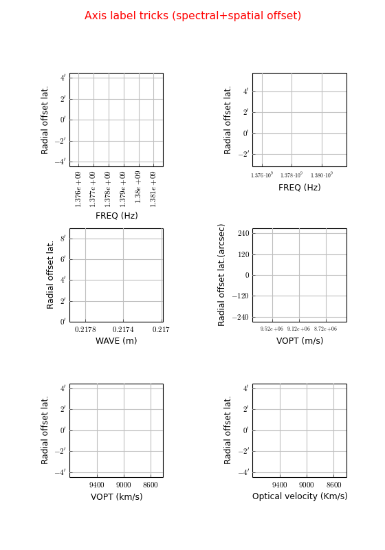
Explanation
The default labeling of the frequency axis is too crowded. We apply the trick to rotate the axis labels grat.setp_tick(plotaxis="bottom", rotation=90)
Here we selected a start value and a step size for the label positions: grat = annim.Graticule(startx="1.378 Ghz", deltax="2 Mhz", starty="53d42m"). We use a special format syntax (%+9e) to tell the plot routines to format the numbers with an exponential: grat.setp_tick(plotaxis="bottom", fontsize=7, fmt='%.3f%+9e')
The spectral axis can be translated into a wave length axis using parameter spectrans. The units change from Hz to m. In the Graticule contructor we use strings for the start value and step size. Then we can use compatible units enter the values. Note that the y axis in our spectral plots is by default an offset axis. For spatial offset axes the reference (value 0) is at the middle of an axis. One can enter a value in grids or world coordinate (enter it as a string) to change this reference point: grat = annim.Graticule(spectrans="WAVE", startx="21.74 cm", deltax="0.04 cm", starty="0.5")
In this plot we use another spectral translation (optical velocity) with a start value and a step size. We changed the units of the offset axis to seconds of arc. grat = annim.Graticule(spectrans="VOPT", startx="9120 km/s", deltax="400 km/s", unitsy="arcsec")
Again with a spectral translation. But the units along the x axis are Km/s. Note that the default units (si units) are used for label positions if there are no units entered. This implies that the value in unitsx does not change the units for startx. It is always save to enter explicit units for startx: grat = annim.Graticule(spectrans="VOPT", startx="9000 km/s", deltax="400 km/s", unitsx="km/s")
You can get even more control if you enter a function or a lambda expression for parameter fun. You have to change the default axis title with method wcsgrat.Graticule.setp_axislabel().
>>> grat.setp_tick(plotaxis="bottom", fmt='%g', fun=lambda x:x/1000.0)
>>> grat.setp_axislabel(plotaxis="bottom", label="Optical velocity (Km/s)")
For the next example we used a FITS file with the following header information:
Axis 1: RA---NCP  from pixel 1 to   100  {crpix=51 crval=-51.2821 cdelt=-0.007166 (DEGREE)}
Axis 2: DEC--NCP  from pixel 1 to   100  {crpix=51 crval=60.1539 cdelt=0.007166 (DEGREE)}
Axis 3: VELO-HEL  from pixel 1 to   101  {crpix=-20 crval=-243 cdelt=4.2 (km/s)}
Example: mu_axnumdemo.py - Show different axes combinations for the same FITS file
1 2 3 4 5 6 7 8 9 10 11 12 13 14 15 16 17 18 19 20 21 22 23 24 25 26 27 28 29 30 31 32 33 34 35 36 37 38 39 40 41 42 43 44 45 46 47 48 49 50 51 52 | from kapteyn import maputils
from matplotlib import pyplot as plt
fitsobj= maputils.FITSimage('ngc6946.fits')
newaspect = 1/5.0 # Needed for XV maps
fig = plt.figure(figsize=(20/2.54, 25/2.54))
fig.subplots_adjust(left=0.18)
labelx = -0.10 # Fix the position in x for labels along y
# fig 1. Spatial map, default axes are 1 & 2
frame1 = fig.add_subplot(4,1,1)
mplim1 = fitsobj.Annotatedimage(frame1)
mplim1.Image()
graticule1 = mplim1.Graticule(deltax=15*2/60.0)
# fig 2. Velocity - Dec
frame2 = fig.add_subplot(4,1,2)
fitsobj.set_imageaxes('vel', 'dec')
mplim2 = fitsobj.Annotatedimage(frame2)
mplim2.Image()
graticule2 = mplim2.Graticule()
graticule2.setp_axislabel(plotaxis='left', xpos=labelx)
# fig 3. Velocity - Dec (Version without offsets)
frame3 = fig.add_subplot(4,1,3)
mplim3 = fitsobj.Annotatedimage(frame3)
mplim3.Image()
graticule3 = mplim3.Graticule(offsety=False)
graticule3.setp_axislabel(plotaxis='left', xpos=labelx)
graticule3.setp_ticklabel(plotaxis="left", fmt='DMs')
# fig 4. Velocity - R.A.
frame4 = fig.add_subplot(4,1,4)
fitsobj.set_imageaxes('vel','ra')
mplim4 = fitsobj.Annotatedimage(frame4)
mplim4.Image()
graticule4 = mplim4.Graticule(offsety=False)
graticule4.setp_axislabel(plotaxis='left', xpos=labelx)
graticule4.setp_ticklabel(plotaxis="left", fmt='HMs')
graticule4.Insidelabels(wcsaxis=0, constval='20h34m',
rotation=90, fontsize=10,
color='r', ha='right')
graticule4.Insidelabels(wcsaxis=1, fontsize=10, fmt="%.2f", color='y')
mplim4.Minortickmarks(graticule4)
#Apply new aspect ratio for the XV maps
mplim2.set_aspectratio(newaspect)
mplim3.set_aspectratio(newaspect)
mplim4.set_aspectratio(newaspect)
maputils.showall()
|
(Source code, png, hires.png, pdf)

We used Matplotlib’s add_subplot() method to create 4 plots in one figure with minimum effort. The top panel shows a plot with the default axis numbers which are 1 and 2. This corresponds to the axis types RA and DEC and therefore the map is a spatial map. The next panel has axis numbers 3 and 2 representing a position-velocity or XV map with DEC as the spatial axis X. The default annotation is offset in spatial distances. The next panel is a copy but we changed the annotation from the default (i.e. offsets) to position labels. This could make sense if the map is unrotated. The bottom panel has RA as the spatial axis X. World coordinate labels are added inside the plot with a special method: wcsgrat.Insidelabels(). These labels are not formatted to hour/min/sec or deg/min/sec for spatial axes.
The two calls to this method need some extra explanation:
graticule4.Insidelabels(wcsaxis=0, constval='20h34m', rotation=90, fontsize=10,
                        color='r', ha='right')
graticule4.Insidelabels(wcsaxis=1, fontsize=10, fmt="%.2f", color='b')
The first statement sets labels that correspond to positions in world coordinates inside a plot. It copies the positions of the velocities, set by the initialization of the graticule object. It plots those labels at a Right Ascension equal to 20h35m which is equal to -51 (=309) degrees. It rotates these labels by an angle of 90 degrees and sets the size, color and alignment of the font. The second statement does something similar for the Right Ascension labels, but it adds also a format for the numbers.
Note also the line:
>>> graticule4 = mplim4.Graticule(offsety=False)
>>> graticule4.setp_ticklabel(plotaxis="left", fmt='HMs')
By default the module would plot labels which are offsets because we have only one spatial axis. We overruled this behaviour with keyword parameter offsety=False. Then we get world coordinates which by default are formatted in hour/minutes/seconds. If we want these labels to be plotted in another format, lets say decimal degrees, then one needs parameter fun to define some transformation and with fmt we set the format for that output, e.g. as in:
>>> graticule4.setp_tick(plotaxis="left", fun=lambda x: x+360, fmt="$%.1f^\circ$")
Finally note that the alignment of the titles along the left axis (which is a Matplotlib method) works in the frame of the graticule. It is important to realize that a maputils plot usually is a stack of matplotlib Axes objects (frames). The graticule object sets these axis labels and therefore we must align them in that frame (which is an attribute of the graticule object) as in:
>>> graticule3.setp_axislabel(plotaxis='left', xpos=labelx)
For information about the Matplotlib specific attributes you should read the documentation at the appropriate class descriptions (http://matplotlib.sourceforge.net).
For images and graticules representing spatial data it is important that the aspect ratio (CDELTy/CDELTx) remains constant if you resize the plot. A graticule object initializes itself with an aspect ratio based on the pixel sizes found in (or derived from) the header. It also calculates an appropriate figure size and size for the actual plot window in normalized device coordinates (i.e. in interval [0,1]). You can use these values in a script to set the relevant values for Matplotlib as we show in the next example.
Example: mu_figuredemo.py - Plot figure in non default aspect ratio
1 2 3 4 5 6 7 8 9 10 11 12 | from kapteyn import maputils
from matplotlib import pyplot as plt
fitsobj = maputils.FITSimage('example1test.fits')
fig = plt.figure(figsize=(5.5,5))
frame = fig.add_axes([0.1, 0.1, 0.8, 0.8])
annim = fitsobj.Annotatedimage(frame)
annim.set_aspectratio(1.2)
grat = annim.Graticule()
maputils.showall()
|
(Source code, png, hires.png, pdf)
Note
For astronomical data we want equal steps in spatial distance in any direction correspond to equal steps in figure size. If one changes the size of the figure interactively, the aspect ratio should not change. To enforce this, the constructor of an object of class maputils.Annotatedimage modifies the input frame so that the aspect ratio is the aspect ratio of the pixels. This aspect ratio is preserved when the size of a window is changed. One can overrule this default by manually setting an aspect ratio with method maputils.Annotatedimage.set_aspectratio() as in:
>>> frame = fig.add_subplot(k,1,1)
>>> mplim = f.Annotatedimage(frame)
>>> mplim.set_aspectratio(0.02)
The number of graticule objects is not restricted to one. One can easily add a second graticule for a different sky system. The next example shows a combination of two graticules for two different sky systems. It demonstrates also the use of attributes to change plot properties.
Example: mu_skyout.py - Combine two graticules in one frame
1 2 3 4 5 6 7 8 9 10 11 12 13 14 15 16 17 18 19 20 21 22 23 24 25 26 27 28 29 30 31 32 33 34 35 36 37 38 39 | from kapteyn.wcs import galactic, equatorial, fk4_no_e, fk5
from kapteyn import maputils
from matplotlib import pylab as plt
# Open FITS file and get header
f = maputils.FITSimage('example1test.fits')
fig = plt.figure(figsize=(6,6))
frame = fig.add_subplot(1,1,1)
annim = f.Annotatedimage(frame)
# Initialize a graticule for this header and set some attributes
grat = annim.Graticule()
grat.setp_gratline(wcsaxis=[0,1],color='g') # Set graticule lines to green
grat.setp_ticklabel(plotaxis=("left","bottom"), color='b',
fontsize=14, fmt="Hms")
grat.setp_tickmark(plotaxis=("left","bottom"), markersize=-10)
# Select another sky system for an overlay
skyout = galactic # Also try: skyout = (equatorial, fk5, 'J3000')
grat2 = annim.Graticule(skyout=skyout, boxsamples=20000)
grat2.setp_axislabel(plotaxis=("top", "right"), label="Galactic l,b",
visible=True)
grat2.set_tickmode(plotaxis=("top", "right"), mode="ALL")
grat2.setp_axislabel(plotaxis="top", color='r')
grat2.setp_axislabel(plotaxis=("left", "bottom"), visible=False)
grat2.setp_ticklabel(plotaxis=("left", "bottom"), visible=False)
grat2.setp_ticklabel(plotaxis=("top", "right"), fmt='Dms')
grat2.setp_gratline(color='r')
# Print coordinate labels inside the plot boundaries
grat2.Insidelabels(wcsaxis=0, color='m', constval=85, fmt='Dms')
grat2.Insidelabels(wcsaxis=1, fmt='Dms')
annim.Pixellabels(plotaxis=("right","top"), gridlines=True,
color='c', markersize=-3, fontsize=7)
annim.plot()
plt.show()
|
(Source code, png, hires.png, pdf)

Explanation:
This plot shows graticules for equatorial coordinates and galactic coordinates in the same figure. The center of the image is the position of the galactic pole. That is why the graticule for the galactic system shows circles. The galactic graticule is also labeled inside the plot using method wcsgrat.Insidelabels() (Note that this is a method derived from class wcsgrat.Graticule and that it is not a method of class maputils.Annotatedimage). To get an impression of arbitrary positions expressed in pixels coordinates, we added pixel coordinate labels for the top and right axes with method maputils.Annotatedimage.Pixellabels().
Plot properties:
- Use attribute boxsamples to get a better estimation of the ranges in galactic coordinates. The default sampling does not sample enough in the neighbourhood of the galactic pole causing a gap in the plot.
- Use method wcsgrat.Graticule.setp_gratline() to change the color of the longitudes and latitudes for the equatorial system.
- Method wcsgrat.Graticule.setp_tickmark() sets for both plot axis (0 == x axis, 1 = y axis) the tick length with markersize. The value is negative to force a tick that points outwards. Also the color and the font size of the tick labels is set. Note that these are Matplotlib keyword arguments.
- With wcsgrat.Graticule.setp_axislabel() we allow galactic coordinate labels and ticks to be plotted along the top and right plot axis. By default, the labels along these axes are set to be invisible, so we need to make them visible with keyword argument visible=True. Also a title is set for these axes.
Note
There is a difference between plot axes and wcs axes. The first always represent a rectangular system with pixels while the system of the graticule lines (wcs axes) usually is curved (sometimes they are even circular. Therefore many plot properties are either associated with one a plot axis and/or a world coordinate axes.
To demonstrate what is possible with spectral coordinates and module wcsgrat we use real interferometer data from a set called mclean.fits. A summary of what can be found in its header:
Axis  1: RA---NCP  from pixel 1 to   512  {crpix=257 crval=178.779 cdelt=-0.0012 (DEGREE)}
Axis  2: DEC--NCP  from pixel 1 to   512  {crpix=257 crval=53.655 cdelt=0.00149716 (DEGREE)}
Axis  3: FREQ-OHEL from pixel 1 to    61  {crpix=30 crval=1.41542E+09 cdelt=-78125 (HZ)}
Its spectral axis number is 3. The type is frequency. The extension tells us that an optical velocity in the heliocentric system is associated with the frequencies. In the header we found that the optical velocity is 1050 Km/s. The header is a legacy GIPSY header and module wcs can interpret it. We require the frequencies to be expressed as wavelengths.
Example: mu_wave.py - Plot a graticule in a position wavelength diagram.
1 2 3 4 5 6 7 8 9 10 11 12 13 14 15 16 17 18 19 20 21 22 23 | from kapteyn import maputils
from matplotlib import pylab as plt
# Make plot window wider if you don't see toolbar info
# Open FITS file and get header
f = maputils.FITSimage('mclean.fits')
f.set_imageaxes('freq','dec')
f.set_limits(pxlim=(35,45))
fig = plt.figure(figsize=f.get_figsize(ysize=12, cm=True))
frame = fig.add_subplot(1,1,1)
annim = f.Annotatedimage(frame)
grat = annim.Graticule(spectrans='WAVE')
grat.setp_ticklabel(plotaxis='bottom', fun=lambda x: x*100, fmt="%.3f")
grat.setp_axislabel(plotaxis='bottom', label="Wavelength (cm)")
grat.setp_gratline(wcsaxis=(0,1), color='g')
annim.Pixellabels(plotaxis=("right","top"), gridlines=False)
annim.plot()
annim.interact_toolbarinfo()
plt.show()
|
(Source code, png, hires.png, pdf)

Explanation:
- With PyFITS we open the fits file on disk and read its header
- A Matplotlib Figure- and Axes instance are made
- The range in pixel coordinates in x is decreased
- A Graticule object is created and FITS axis 3 (FREQ) is associated with x and FITS axis 2 (DEC) with y. The spectral axis is expressed in wavelengths with method wcs.Projection.spectra(). Note that we omitted a code for the conversion algorithm and instead entered three question marks so that the spectra() method tries to find the appropriate code.
- The tick labels along the x axis (the wavelengths) are formatted. The S.I. unit is meter, but we want it to be plotted in cm. A function to convert the values is given with fun=lambda x: x*100. A format for the printed numbers is given with: fmt=”%.3f”
Note
The spatial axis is expressed in offsets. By default it starts with an offset equal to zero in the middle of the plot. Then a suitable step size is calculated and the corresponding labels are plotted. For spatial offsets we need also a value for the missing spatial axis. If not specified with parameter mixpix in the constructor of class Graticule, a default value is assumed equal to CRPIX corresponding to the missing spatial axis (or 1 if CRPIX is outside interval [1,NAXIS])
For the next example we use the same FITS file (mclean.fits).
Example: mu_spectraltypes.py - Plot grid lines for different spectral translations
1 2 3 4 5 6 7 8 9 10 11 12 13 14 15 16 17 18 19 20 21 22 23 24 25 26 27 28 29 30 31 32 33 34 35 36 37 38 39 40 41 42 43 44 45 46 47 48 | from kapteyn import maputils
from matplotlib import pyplot as plt
# Read header of FITS file
f = maputils.FITSimage('mclean.fits')
# Matplotlib
fig = plt.figure(figsize=(7,10))
fig.subplots_adjust(left=0.12, bottom=0.05, right=0.97,
top=0.97, wspace=0.22, hspace=0.90)
fig.text(0.05,0.5,"Radial offset latitude", rotation=90,
fontsize=14, va='center')
# Get the projection object to get allowed spectral translations
altspec = f.proj.altspec
crpix = f.proj.crpix[f.proj.specaxnum-1]
altspec.insert(0, (None, '')) # Add native to list
k = len(altspec) + 1
frame = fig.add_subplot(k,1,1)
# Limit range in x to neighbourhood of CRPIX
xlim = (crpix-5, crpix+5)
f.set_imageaxes(3,2)
f.set_limits(pxlim=xlim)
mplim = f.Annotatedimage(frame)
mplim.set_aspectratio(0.002)
print "Native system", f.proj.ctype[f.proj.specaxnum-1], f.proj.cunit[f.proj.specaxnum-1],
print "Spectral translations"
for i, ast in enumerate(altspec):
print i, ast
frame = fig.add_subplot(k,1,i+1)
mplim = f.Annotatedimage(frame)
mplim.set_aspectratio(0.002)
grat = mplim.Graticule(spectrans=ast[0], boxsamples=3)
grat.setp_ticklabel(plotaxis="bottom", fmt="%g")
unit = ast[1]
ctype = ast[0]
if ctype == None:
ctype = "Frequency (Hz) without translation"
grat.setp_axislabel(plotaxis="bottom",
label=ctype+' '+unit, color='b', fontsize=10)
grat.setp_axislabel("left", visible=False)
grat.setp_ticklabel(wcsaxis=(0,1), fontsize='8')
mplim.plot()
plt.show()
|
(Source code, png, hires.png, pdf)
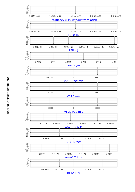
Explanation:
- With PyFITS we open the FITS file on disk and read its header
- We created a wcs.Projection object for this header to get a list with allowed spectral translations (attribute altspec). We need this list before we create the graticules
- Matplotlib Figure- and Axes instances are made
- The native FREQ axis (top figure) differs from the FREQ axis in the next plot, because a legacy header was found and its freqencies were transformed to a barycentric/heliocentric system.
Rulers are objects derived from an Annimatedimage object. The class description is found at rulers.Ruler. A ruler is always plotted as a straight line, whatever the projection (so it doesn’t necessarily follow graticule lines). A ruler plots ticks and labels and the spatial distance between any two ticks is a constant given by a user in parameter step. This makes rulers ideal to put nearby a feature in your map to give an idea of the physical size of that feature. Rulers can be plotted in maps with one or two spatial axes. They are either defined by a start- and an end point (in pixel or world coordinates) or by a start point and a size and angle (w.r.t. the North). This size and angle are defined on a sphere.
Note
Rulers, Beams and Markers can be positioned using either pixel coordinates or world coordinates in a string. See the examples in module positions.
Example: mu_manyrulers.py - Ruler demonstration
1 2 3 4 5 6 7 8 9 10 11 12 13 14 15 16 17 18 19 20 21 22 23 24 25 26 27 28 29 30 31 32 33 34 35 36 37 38 39 40 41 42 43 44 45 46 47 48 49 50 51 52 53 54 55 56 57 58 59 60 61 62 63 64 65 66 67 68 | from kapteyn import maputils
from matplotlib import pylab as plt
header = {'NAXIS' : 2, 'NAXIS1': 800, 'NAXIS2': 800,
'CTYPE1':'RA---TAN',
'CRVAL1': 0.0, 'CRPIX1' : 1, 'CUNIT1' : 'deg', 'CDELT1' : -0.05,
'CTYPE2':'DEC--TAN',
'CRVAL2': 0.0, 'CRPIX2' : 1, 'CUNIT2' : 'deg', 'CDELT2' : 0.05,
}
fitsobject = maputils.FITSimage(externalheader=header)
fig = plt.figure()
frame = fig.add_axes([0.1,0.1, 0.82,0.82])
annim = fitsobject.Annotatedimage(frame)
grat = annim.Graticule(header)
x1 = 10; y1 = 1
x2 = 10; y2 = annim.pylim[1]
ruler1 = annim.Ruler(x1=x1, y1=y1, x2=x2, y2=y2, lambda0=0.0, step=1.0)
ruler1.setp_label(color='g')
x1 = x2 = annim.pxlim[1]
ruler2 = annim.Ruler(x1=x1, y1=y1, x2=x2, y2=y2, lambda0=0.5, step=2.0,
fmt='%3d', mscale=-1.5, fliplabelside=True)
ruler2.setp_label(ha='left', va='center', color='b', clip_on=False)
ruler3 = annim.Ruler(x1=23*15, y1=30, x2=22*15, y2=15, lambda0=0.0,
step=2, world=True,
units='deg', addangle=90)
ruler3.setp_label(color='r')
ruler4 = annim.Ruler(pos1="23h0m 15d0m", pos2="22h0m 30d0m", lambda0=0.0,
step=1,
fmt="%4.0f^\prime",
fun=lambda x: x*60.0, addangle=0)
ruler4.setp_line(color='g')
ruler4.setp_label(color='m')
ruler5 = annim.Ruler(x1=1, y1=800, x2=800, y2=800, lambda0=0.5, step=2,
fmt="%4.1f", addangle=90)
ruler5.setp_label(color='c')
ruler6 = annim.Ruler(pos1="23h0m 15d0m", rulersize=15, step=2,
units='deg', lambda0=0, fliplabelside=True)
ruler6.setp_label(color='b')
ruler6.set_title("Size in deg", fontsize=10)
ruler7 = annim.Ruler(pos1="23h0m 30d0m", rulersize=5, rulerangle=90, step=1,
units='deg', lambda0=0)
ruler7.setp_label(color='#ffbb33')
ruler8 = annim.Ruler(pos1="23h0m 15d0m", rulersize=5, rulerangle=10, step=1.25,
units='deg', lambda0=0, fmt="%02g", fun=lambda x: x*8)
ruler8.setp_label(color='#3322ff')
ruler8.set_title("Size in kpc", fontsize=10)
# Increase size and lambda a bit to get all the labels
# from 5 to 0 and to 5 again plotted
# Show LaTeX in ruler label
ruler9 = annim.Ruler(pos1="23h0m 10d0m", rulersize=10.1, rulerangle=90, step=1,
units='deg', lambda0=0.51)
ruler9.setp_label(color='#33ff22')
ruler9.set_title("$\lambda = 0.5$", fontsize=10)
annim.plot()
annim.interact_toolbarinfo()
annim.interact_writepos()
plt.show()
|
(Source code, png, hires.png, pdf)
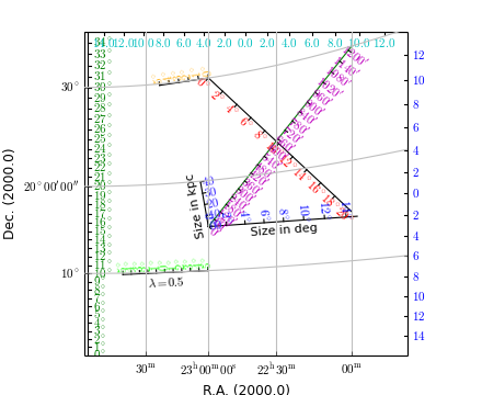
Ruler tick labels can be formatted so that we can adjust the values near the ruler ticks with parameter fmt. With parameter fun it is possible to convert the spatial distance to some other physical quantity. Parameter fun accepts a function or a lambda expression. You can use method rulers.Ruler.set_title() to annotate alternative units. Note that the keyword arguments for this method are the same as for Matplotlib’s set_title() method.
In the next plot we want offsets to be plotted in arcminutes.
Example: mu_arcminrulers.py - Rulers with non default labels
1 2 3 4 5 6 7 8 9 10 11 12 13 14 15 16 17 18 19 20 21 22 23 24 25 26 27 28 29 30 31 32 33 34 35 36 37 38 39 40 41 42 | from kapteyn import maputils
from matplotlib import pyplot as plt
header = {'NAXIS' : 2, 'NAXIS1': 100, 'NAXIS2': 100,
'CTYPE1' : 'RA---TAN',
'CRVAL1' : 80.0, 'CRPIX1' : 1,
'CUNIT1' : 'arcmin', 'CDELT1' : -0.5,
'CTYPE2' : 'DEC--TAN',
'CRVAL2' : 400.0, 'CRPIX2' : 1,
'CUNIT2' : 'arcmin', 'CDELT2' : 0.5,
'CROTA2' : 30.0
}
f = maputils.FITSimage(externalheader=header)
fig = plt.figure()
frame = fig.add_axes([0.1,0.15,0.8,0.75])
annim = f.Annotatedimage(frame)
grat = annim.Graticule()
grat.setp_ticklabel(plotaxis='bottom', rotation=90)
grat.setp_ticklabel(fmt='s') # Suppress the seconds in all labels
# Use pixel limits attributes of the FITSimage object
xmax = annim.pxlim[1]+0.5; ymax = annim.pylim[1]+0.5
annim.Ruler(x1=xmax, y1=0.5, x2=xmax, y2=ymax, lambda0=0.5, step=5.0/60.0,
fun=lambda x: x*60.0, fmt="%4.0f^\prime",
fliplabelside=True, color='r')
# The wcs methods that convert between pixels and world
# coordinates expect input in degrees whatever the units in the
# header are (e.g. arcsec, arcmin).
annim.Ruler(x1=60/60.0, y1=390/60.0, x2=60/60.0, y2=420/60.0,
lambda0=0.0, step=5.0/60, world=True,
fun=lambda x: x*60.0, fmt="%4.0f^\prime", color='g')
annim.Ruler(pos1='0h3m30s 6d30m', pos2='0h3m30s 7d0m',
lambda0=0.0, step=5.0,
units='arcmin', color='c')
annim.plot()
plt.show()
|
(Source code, png, hires.png, pdf)
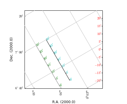
It is possible to put a ruler in a map with only one spatial coordinate (as long there is a matching axis in the header) like a Position-Velocity diagram (sometimes also called XV maps). It will take the pixel coordinate of the slice as a constant so even for XV maps we have reliable offsets. In the next example we created two rulers. The red ruler is in fact the same as the Y-axis offset labeling. The blue ruler show the same offsets in horizontal direction. That is because only the horizontal direction is spatial. Such a ruler is probably not very useful but is a nice demonstration of the flexibility of method maputils.Annotatedimage.Ruler().
Note that we set Matplotlib’s clip_on to True because if we pan the image in Matplotlib we don’t want the labels to be visible outside the border of the frame.
Example: mu_xvruler.py - Ruler in a XV map
1 2 3 4 5 6 7 8 9 10 11 12 13 14 15 16 17 18 19 20 21 22 23 24 25 26 27 28 29 30 31 32 33 34 35 | from kapteyn import maputils
from matplotlib import pylab as plt
# Open FITS file and get header
f = maputils.FITSimage('ngc6946.fits')
f.set_imageaxes(3,2) # X axis is velocity, y axis is declination
fig = plt.figure(figsize=f.get_figsize(xsize=15, cm=True))
frame = fig.add_subplot(1,1,1)
annim = f.Annotatedimage(frame)
# Velocity - Dec
grat = annim.Graticule()
grat.setp_axislabel("right", label="Offset (Arcmin.)", visible=True)
xmax = annim.pxlim[1]+0.5; ymax = annim.pylim[1]+0.5
ruler = annim.Ruler(x1=xmax, y1=0.5, x2=xmax, y2=ymax,
lambda0 = 0.5, step=5.0/60.0,
fun=lambda x: x*60.0, fmt="%4.0f^\prime",
fliplabelside=True)
ruler.setp_line(lw=2, color='r')
ruler.setp_label(color='r')
ruler2 = annim.Ruler(x1=0.5, y1=0.5, x2=xmax, y2=ymax, lambda0 = 0.5,
step=5.0/60.0,
fun=lambda x: x*60.0, fmt="%4.0f^\prime",
fliplabelside=True)
ruler2.setp_line(lw=2, color='b')
ruler2.setp_label(color='b')
annim.plot()
annim.interact_writepos()
plt.show()
|
(Source code, png, hires.png, pdf)
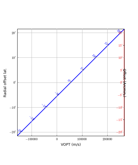
Example: mu_simplecontours.py - Simple plot with contour lines only
1 2 3 4 5 6 7 8 9 10 11 12 13 | from kapteyn import maputils
from matplotlib import pyplot as plt
fitsobj = maputils.FITSimage("m101.fits")
fitsobj.set_limits((200,400), (200,400))
annim = fitsobj.Annotatedimage()
cont = annim.Contours()
annim.plot()
print "Levels=", cont.clevels
plt.show()
|
(Source code, png, hires.png, pdf)
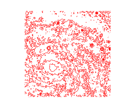
The example above shows how to plot contours without plotting an image. It also shows how one can retrieve the contour levels that are calculated as a default because no levels were specified.
Next we demonstrate how to use the three Matplotlib keyword arguments to set some global properties of the contours:
Example: mu_contourlinestyles.py - Setting global colors and line styles/widths
1 2 3 4 5 6 7 8 9 10 11 12 13 14 15 | from kapteyn import maputils
from matplotlib import pyplot as plt
fitsobj = maputils.FITSimage("m101.fits")
fitsobj.set_limits((200,400), (200,400))
annim = fitsobj.Annotatedimage()
annim.Image(alpha=0.5)
cont = annim.Contours(linestyles=('solid', 'dashed', 'dashdot', 'dotted'),
linewidths=(2,3,4), colors=('r','g','b','m'))
annim.plot()
print "Levels=", cont.clevels
plt.show()
|
(Source code, png, hires.png, pdf)
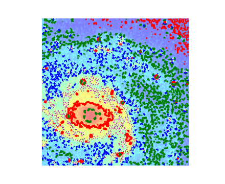
Example: mu_annotatedcontours.py - Add annotation to contours
1 2 3 4 5 6 7 8 9 10 11 12 13 14 15 16 17 18 19 20 21 22 | from kapteyn import maputils
from matplotlib import pyplot as plt
f = maputils.FITSimage("m101.fits")
f.set_limits(pxlim=(200,350), pylim=(200,350))
fig = plt.figure()
frame = fig.add_subplot(1,1,1)
mplim = f.Annotatedimage(frame)
cont = mplim.Contours(levels=range(10000,16000,1000))
cont.setp_contour(linewidth=1)
cont.setp_contour(levels=11000, color='g', linewidth=3)
# Second contour set only for labels
cont2 = mplim.Contours(levels=(8000,9000,10000,11000))
cont2.setp_label(11000, colors='b', fontsize=14, fmt="%.3f")
cont2.setp_label(fontsize=10, fmt="%g \lambda")
mplim.plot()
plt.show()
|
(Source code, png, hires.png, pdf)
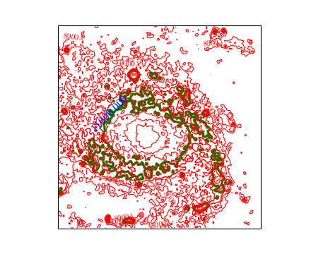
The plot shows two sets of contours. The first step is to plot all contours in a straightforward way. The second is to plot contours with annotation. For this second set we don’t see any contours if a label could not be fitted that’s why we first plot all the contours. Note that now we can use the properties methods for single contours because we can identify these contours by their corresponding level.
Example: mu_negativecontours.py - Contours with different line styles for negative values
1 2 3 4 5 6 7 8 9 10 11 12 13 14 15 16 | """ Show contour lines with different lines styles """
from kapteyn import maputils
from matplotlib import pyplot as plt
f = maputils.FITSimage("RAxDEC.fits")
fig = plt.figure(figsize=(8,6))
frame = fig.add_subplot(1,1,1)
mplim = f.Annotatedimage(frame)
cont = mplim.Contours(levels=[-500,-300, 0, 300, 500], negative="dotted")
cont.setp_label()
mplim.plot()
mplim.interact_toolbarinfo()
plt.show()
|
(Source code, png, hires.png, pdf)
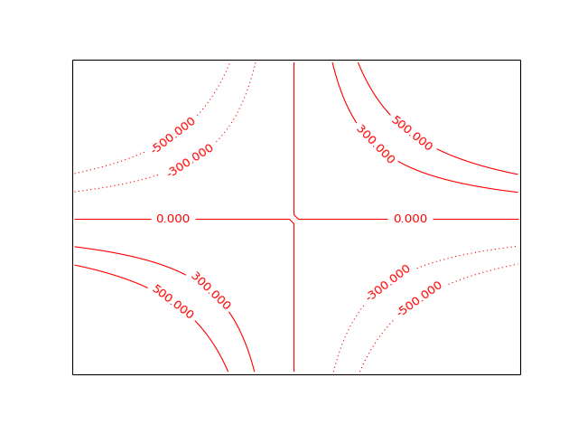
A colorbar is an image which shows colors and values which correspond to these colors. It is a tool that helps you to inspect the values in an image. The distribution of the colors depends on the selected color map and the selected clip levels. Next example shows how to setup a colorbar. The default position is calculated by Matplotlib. It borrows space from the current frame depending on the orientation (‘vertical’ or ‘horizontal’).
Example: mu_colbar.py - Add colorbar to plot
1 2 3 4 5 6 7 8 9 10 11 12 | from kapteyn import maputils
from matplotlib import pyplot as plt
fitsobj = maputils.FITSimage("m101.fits")
mplim = fitsobj.Annotatedimage(cmap="spectral")
mplim.Image()
units = r'$ergs/(sec.cm^2)$'
colbar = mplim.Colorbar(fontsize=8)
colbar.set_label(label=units, fontsize=24)
mplim.plot()
plt.show()
|
(Source code, png, hires.png, pdf)

If you want more control over the position and size of the colorbar then specify a frame for the colorbar. In the next example we prepared a frame for both the image and the colorbar. If you don’t enter a figure size, it can happen that the figure does not provide enough space in either width or height. In the example we want the colorbar to be as big as the width of the image. This will be a problem with the default figure size so we provided some extra space in height with figsize=:
Example: mu_colbarframe.py - Add colorbar with user’s frame to plot
1 2 3 4 5 6 7 8 9 10 11 12 13 14 15 16 17 | from kapteyn import maputils
from matplotlib import pyplot as plt
fitsobj = maputils.FITSimage("m101.fits")
fig = plt.figure(figsize=(5,7.5))
#fig = plt.figure()
frame = fig.add_axes((0.1, 0.2, 0.8, 0.8))
cbframe = fig.add_axes((0.1, 0.1, 0.8, 0.1))
annim = fitsobj.Annotatedimage(cmap="Accent", clipmin=8000, frame=frame)
annim.Image()
units = r'$ergs/(sec.cm^2)$'
colbar = annim.Colorbar(fontsize=8, orientation='horizontal', frame=cbframe)
colbar.set_label(label=units, fontsize=24)
annim.plot()
annim.interact_imagecolors()
plt.show()
|
(Source code, png, hires.png, pdf)
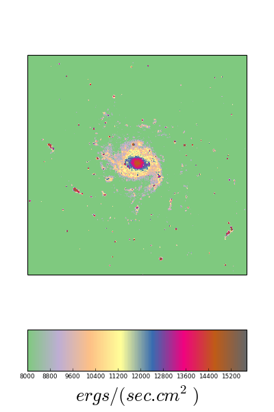
Note that we entered a colormap (case sensitive names!) and a value for the lower clip value (below which all image pixels get the same color). The clip for the maximum is not entered so the default will be taken which is the maximum intensity in your image.
Note also that we added interaction to set other colormaps and to change the relation between colors and image values. Interaction is a topic in a later section of this tutorial.
Usually one associates colorbars with images but it can also be used in combination with contours. We demonstrate the use of Matplotlib’s keyword parameters visible=False to make an image invisible. However, to make the contents of the colorbar invisible one should use alpha=0.0 but we implemented keyword visible to simulate this effect.
Example: mu_colbarwithlines.py - Add lines representing contours in plot to dummy colorbar
1 2 3 4 5 6 7 8 9 10 11 12 13 14 15 16 17 18 19 20 21 22 23 24 25 26 27 28 29 30 31 32 33 34 35 36 37 38 39 40 41 42 43 44 45 46 47 48 49 50 51 52 53 54 55 56 57 58 59 60 61 62 63 64 65 66 67 68 69 | from kapteyn import maputils
from matplotlib import pyplot as plt
f = maputils.FITSimage("m101.fits")
limy = limx=(160,360)
f.set_limits(limx,limy)
rows = 3
cols = 2
fig = plt.figure(figsize=(8,10))
frame = fig.add_subplot(rows,cols,1)
mplim = f.Annotatedimage(frame, cmap="spectral")
cont = mplim.Contours()
mplim.Colorbar(clines=True, fontsize=8, linewidths=5) # show only cont. lines
mplim.plot()
# Levels only known after plotted
print "Proposed levels:", cont.clevels
frame = fig.add_subplot(rows,cols,2)
mplim = f.Annotatedimage(frame, cmap="spectral")
cont = mplim.Contours(filled=True)
mplim.Colorbar(clines=True, fontsize=8) # show only cont. lines
mplim.plot()
frame = fig.add_subplot(rows,cols,3)
mplim = f.Annotatedimage(frame, cmap="spectral")
mplim.Image()
cont = mplim.Contours(colors='w', linewidths=1)
mplim.Colorbar(clines=True, ticks=(4000,8000,12000))
mplim.plot()
mplim.interact_imagecolors()
frame = fig.add_subplot(rows,cols,4)
mplim = f.Annotatedimage(frame, cmap="spectral")
mplim.Image()
# Give each contour its own color, instead of borrowing from the colormap
cont = mplim.Contours(levels=(6000,8000,10000,12000),
colors=('w','g','b', 'c'))
cont.setp_contour(levels=8000, color='m', linewidth=2)
mplim.Colorbar(clines=True, ticks=(4000,8000,12000), linewidths=6)
mplim.plot()
mplim.interact_imagecolors()
mplim.interact_toolbarinfo()
frame = fig.add_subplot(rows,cols,5)
mplim = f.Annotatedimage(frame, cmap="mousse.lut")
mplim.Image()
cont = mplim.Contours()
mplim.Colorbar(clines=True, orientation="horizontal", ticks=(4000,8000,12000))
mplim.plot()
mplim.interact_imagecolors()
mplim.interact_toolbarinfo()
# With given levels
frame = fig.add_subplot(rows,cols,6)
levels = (10000,11000,12000,13000)
mplim = f.Annotatedimage(frame, cmap="mousse.lut",
clipmin=min(levels)-500,
clipmax=max(levels)+500)
mplim.Image()
cont = mplim.Contours(levels=levels)
mplim.Colorbar(clines=True, orientation="horizontal",
ticks=levels)
mplim.plot()
mplim.interact_imagecolors()
mplim.interact_toolbarinfo()
plt.show()
|
(Source code, png, hires.png, pdf)

In Matplotlib the axes in a frame are coupled. To get uncoupled axes a we stack frames at the same location. For each frame one can change properties of the pixel coordinate labels separately. The trick is implemented in a number of methods, but in the methods of class maputils.Pixellabels it is easy to demonstrate that it works. In the example we defined 4 plot axes for which we want to draw pixel coordinate labels. The constructor uses Matplotlib defaults but these can be overruled by parameters major and minor. These are numbers for which n*major major ticks and labels are plotted and m*minor minor ticks. Note that the default in Matplotlib is not to plot minor tick marks.
Example: mu_pixellabels.py - Add annotation for pixel coordinates
1 2 3 4 5 6 7 8 9 10 11 12 13 14 15 16 17 18 19 20 21 | from kapteyn import maputils
from matplotlib import pyplot as plt
fig = plt.figure(figsize=(4,4))
frame = fig.add_subplot(1,1,1)
fitsobject = maputils.FITSimage("m101.fits")
annim = fitsobject.Annotatedimage(frame)
annim.Pixellabels(plotaxis="bottom", major=200, minor=10, color="r")
pl2 = annim.Pixellabels(plotaxis="right", color="b", markersize=10,
gridlines=True)
pl2.setp_marker(markersize=+15, color='b', markeredgewidth=2)
pl3 = annim.Pixellabels(plotaxis="top", color='g',
gridlines=False)
pl3.setp_marker(markersize=-10)
pl3.setp_label(rotation=90)
pl4 = annim.Pixellabels(plotaxis="left", major=150, minor=25)
pl4.setp_label(fontsize=10)
annim.plot()
plt.show()
|
(Source code, png, hires.png, pdf)
Objects from class Beam are graphical representations of the resolution of an instrument. The beam is plotted at a center position entered as a string that represents a position or as two world coordinates. The major axis of the beam is the FWHM of longest distance between two opposite points on the ellipse. The angle between the major axis and the North is the position angle of the beam. See also maputils.Annotatedimage.Beam().
Note
Rulers, Beams and Markers are positioned using either pixel coordinates or world coordinates. See the examples in module positions.
In the next example we added two rulers to prove that the sizes of plotted ellipse are indeed the correct values on a sphere. Note also the use of parameter units to set the FWHM’s to minutes of arc.
Example: mu_beam.py - Plot an ellipse representing a beam
1 2 3 4 5 6 7 8 9 10 11 12 13 14 15 16 17 18 19 20 21 22 23 24 25 26 27 28 29 30 31 32 33 34 35 36 37 38 39 40 41 42 43 44 45 46 47 48 49 50 51 52 | from kapteyn import maputils
from matplotlib import pyplot as plt
from math import cos, radians
fitsobj = maputils.FITSimage('m101.fits')
annim = fitsobj.Annotatedimage()
annim.Image()
grat = annim.Graticule()
grat.setp_ticklabel(wcsaxis=1, fmt='s') # Exclude seconds in label
# beam = annim.Beam(210.9619, 54.261039, 0.01, 0.01, 0, hatch='*')
# Hatching does not work in mpl 0.98.3
fwhm_maj = 5/60.0 # arcmin to degrees
fwhm_min = 4/60.0
lat = 54.347395233845
lon = 210.80254413455
beam = annim.Beam(fwhm_maj, fwhm_min, 90, xc=lon, yc=lat,
fc='g', fill=True, alpha=0.6)
pos = '210.80254413455 deg, 54.347395233845 deg'
beam = annim.Beam(7, 4, units='arcmin', pos=pos, fc='m', fill=True,
alpha=0.6)
pos = '14h03m12.6105s 54d20m50.622s'
beam = annim.Beam(fwhm_maj, fwhm_min, pos=pos, fc='y', fill=True, alpha=0.6)
pos = 'ga 102.0354152 {} 59.7725125'
beam = annim.Beam(fwhm_maj, fwhm_min, pos=pos, fc='g', fill=True, alpha=0.6)
pos = 'ga 102d02m07.494s {} 59.7725125'
beam = annim.Beam(fwhm_maj, fwhm_min, pos=pos, fc='b', fill=True, alpha=0.6)
pos = '{ecliptic,fk4, j2000} 174.3674627 {} 59.7961737'
beam = annim.Beam(fwhm_maj, fwhm_min, pos=pos, fc='r', fill=True, alpha=0.6)
pos = '{eq, fk4-no-e, B1950} 14h01m26.4501s {} 54d35m13.480s'
beam = annim.Beam(fwhm_maj, fwhm_min, pos=pos, fc='c', fill=True, alpha=0.6)
pos = '{eq, fk4-no-e, B1950, F24/04/55} 14h01m26.4482s {} 54d35m13.460s'
beam = annim.Beam(fwhm_maj, fwhm_min, pos=pos, fc='c', fill=True, alpha=0.6)
pos = '{ecl} 174.367764 {} 59.79623457'
beam = annim.Beam(fwhm_maj, fwhm_min, pos=pos, fc='c', fill=True, alpha=0.6)
pos = '53 58' # Pixels
beam = annim.Beam(0.04, 0.02, pa=30, pos=pos, fc='y', fill=True, alpha=0.4)
pos = '14h03m12.6105s 58'
beam = annim.Beam(0.04, 0.02, pa=-30, pos=pos, fc='y', fill=True, alpha=0.4)
annim.Ruler(x1=lon, y1=lat, x2=lon+fwhm_min/1.99/cos(radians(54.20)), y2=lat,
world=True, step=1, lambda0=0.0, units='arcmin', color='r')
annim.Ruler(x1=lon, y1=lat, x2=lon, y2=lat+fwhm_maj/1.99, world=True,
step=1, lambda0=0.0, units='arcmin', color='b')
annim.plot()
annim.interact_toolbarinfo()
annim.interact_imagecolors()
plt.show()
|
(Source code, png, hires.png, pdf)

Sometimes there are features in an image that you want to mark with a symbol. In other cases you want to plot positions from an external source (file or database etc.). Then you use objects from class maputils.Annotatedimage.Marker(). The use is straightforward. Positions can be entered in different formats: as pixel coordinates, as world coordinates or as strings with position information (see module positions).
Note
Rulers, Beams and Markers are positioned using either pixel coordinates or world coordinates. See the examples in module positions.
Note the use of Matplotlib keyword arguments to set the properties of the marker symbols. The most important are:
>>> marker=
>>> markersize=
>>> markeredgewidth=
>>> markeredgecolor=
>>> markerfacecolor=
Example: mu_markers.py - Different ways to define marker positions
1 2 3 4 5 6 7 8 9 10 11 12 13 14 15 16 17 18 19 20 21 22 23 24 25 26 27 28 29 30 31 32 33 34 35 36 37 38 39 40 41 42 43 | from kapteyn import maputils, tabarray
from matplotlib import pyplot as plt
import numpy
f = maputils.FITSimage("m101.fits")
fig = plt.figure()
frame = fig.add_subplot(1,1,1)
annim = f.Annotatedimage(frame, cmap="binary")
annim.Image()
grat = annim.Graticule()
#annim.Marker(pos="210.80 deg 54.34 deg", marker='o', color='b')
annim.Marker(pos="pc", marker='o', markersize=10, color='r')
annim.Marker(pos="14h03m30 54d20m", marker='o', color='y')
annim.Marker(pos="ga 102.035415152 ga 59.772512522", marker='+',
markersize=20, markeredgewidth=2, color='m')
annim.Marker(pos="{ecl,fk4,J2000} 174.367462651 {} 59.796173724",
marker='x', markersize=20, markeredgewidth=2, color='g')
annim.Marker(pos="{eq,fk4-no-e,B1950,F24/04/55} 210.360200881 {} 54.587072397",
marker='o', markersize=25, markeredgewidth=2, color='c',
alpha=0.4)
# Use pos= keyword argument to enter sequence of
# positions in pixel coordinates. The syntax is described
# in the module positions.py
pos = "200+20*sin([100:199]/20), range(100,200)"
annim.Marker(pos=pos, marker='o', color='r')
# Use x= and y= keyword arguments to enter sequence of
# positions in pixel coordinates. Note that this is not parsed by
# module positions.py. Here we need list comprehension to
# get the same effect.
xp = [400+20*numpy.sin(x/20.0) for x in range(100,200)]
yp = range(100,200)
annim.Marker(x=xp, y=yp, mode='pixels', marker='o', color='g')
xp = yp = 150
annim.Marker(x=xp, y=yp, mode='pixels', marker='+', color='b')
annim.plot()
annim.interact_imagecolors()
annim.interact_toolbarinfo()
plt.show()
|
(Source code, png, hires.png, pdf)

Sometimes one needs to plot a shape which represents an area in the sky. Such a shape can be a small ellipse which represents the beam of a radio telescope or it is a rectangle representing a footprint of a survey. These shapes (ellipse, circle, rectangle, square, regular polygon) have a prescription. For example a circle is composed of a number of vertices with a constant distance to a center and all the vertices define a different angle. If you want to plot such a shape onto a projection of a sphere you need to recalculate the vertices so that for a given center (lon_c,lat_c) the set of distances and angles are preserved on the sphere. By distances we mean the distance along a great circle and not along a parallel.
So what we do is calculate vertices of an ellipse/rectangle/regular polygon in a plane and the center of the shape is at (0,0). For a sample of points on the shape we calculate the distance of the perimeter as function of the angle. Then with spherical trigonometry we solve for the missing (lon,lat) in the triangle (lon_c,lat_c)-Pole-(lon,lat). This is the position for which the distance along a great circle is the required one and also the angle is the required one.
Assume a triangle on a sphere connecting two positions Q1 with \((\alpha_1, \delta1)\) and Q2 with \((\alpha_2, \delta2)\) and on the sphere Q2 is situated to the left of Q1. Q1 is the new center of the polygon. P is the pole and Q2 the position we need to find. This position has distance d along a great circle connecting Q1 and Q2 and the angle PQ1Q2 is the required angle \(\alpha\). The sides of the triangle are \((90-\delta_1)\) and \((90-\delta_2)\)
Then the distance between Q1 and Q2 is given by:
from which we calculate \(\cos(\alpha_2-\alpha_1)\)
Angle Q1PQ2 is equal to \(\alpha_2-\alpha_1\). For this angle we have the sine formula:
so that:
With \(\cos(\alpha_2-\alpha_1)\) and the value of \(\sin(\alpha_2-\alpha_1)\) we derive an unambiguous value for \(\alpha_2-\alpha_1\) and because we started with \(\alpha_1\) we derive a value for \(\alpha_2\).
The angle PQ1Q2 is \(\alpha\). This is not the astronomical convention, but that doesn’t matter because we use the same definition for an angle in the ‘flat space’ polygon. For this situation we have another cosine rule:
or:
which gives \(\delta_2\) and we found longitude and latitude \((\alpha_2,\delta_2)\) of the transformed ‘flat space’ coordinate. The set of transformed vertices in world coordinates are then transformed to pixels which involves the projection of a map.
The next example shows some shapes plotted in a map of a part of the sky.
Example: mu_skypolygons.py - ‘Sky polygons’ in M101
1 2 3 4 5 6 7 8 9 10 11 12 13 14 15 16 17 18 19 20 21 22 23 24 25 26 27 28 29 30 31 32 33 34 35 36 37 38 39 40 41 42 43 44 45 46 47 48 49 50 51 52 53 | from kapteyn import maputils
from matplotlib import pyplot as plt
f = maputils.FITSimage("m101.fits")
fig = plt.figure()
frame = fig.add_subplot(1,1,1)
annim = f.Annotatedimage(frame, cmap='gist_yarg')
annim.Image()
grat = annim.Graticule()
grat.setp_gratline(color='0.75')
# Ellipse centered on crossing of two graticule lines
annim.Skypolygon("ellipse", cpos="14h03m 54d20m", major=100, minor=50,
pa=-30.0, units='arcsec', fill=False)
# Ellipse at given pixel coordinates
annim.Skypolygon("ellipse", cpos="10 10", major=100, minor=50,
pa=-30.0, units='arcsec', fc='c')
# Circle with radius in arc minutes
annim.Skypolygon("ellipse", cpos="210.938480 deg 54.269206 deg",
major=1.50, minor=1.50, units='arcmin',
fc='g', alpha=0.3, lw=3, ec='r')
# Rectangle at the projection center
annim.Skypolygon("rectangle", cpos="pc pc", major=200, minor=50,
pa=30.0, units='arcsec', ec='g', fc='b', alpha=0.3)
# Regular polygon with 6 angles at some position in galactic coordinates
annim.Skypolygon("npoly", cpos="ga 102d11m35.239s ga 59d50m25.734",
major=150, nangles=6,
units='arcsec', ec='g', fc='y', alpha=0.3)
# Regular polygon
annim.Skypolygon("npolygon", cpos="ga 102.0354152 ga 59.7725125",
major=150, nangles=3,
units='arcsec', ec='g', fc='y', alpha=0.3)
lons = [210.969423, 210.984761, 210.969841, 210.934896, 210.894589,
210.859949, 210.821008, 210.822413, 210.872040]
lats = [54.440575, 54.420249, 54.400778, 54.388611, 54.390166,
54.396241, 54.416029, 54.436244, 54.454230]
annim.Skypolygon(prescription=None, lons=lons, lats=lats, fc='r', alpha=0.3)
annim.plot()
annim.interact_toolbarinfo()
annim.interact_imagecolors()
annim.interact_writepos(wcsfmt="%f",zfmt=None, pixfmt=None, hmsdms=False)
plt.show()
|
(Source code, png, hires.png, pdf)

In ‘all sky’ plots the results can be a little surprising. For the family of cylindrical projections we give a number of examples.
Example: mu_skypolygons_allsky.py - ‘Sky polygons’ in a number of cylindrical projections
1 2 3 4 5 6 7 8 9 10 11 12 13 14 15 16 17 18 19 20 21 22 23 24 25 26 27 28 29 30 31 32 33 34 35 36 37 38 39 40 41 42 43 44 45 46 47 48 49 50 51 52 53 54 55 56 57 58 59 60 61 62 63 64 65 66 67 68 69 70 71 72 73 74 75 76 77 78 79 80 81 82 83 84 85 86 87 88 89 90 91 92 93 94 95 96 97 98 99 100 101 102 103 104 | from kapteyn import maputils
from matplotlib import pyplot as plt
import numpy
def shapes(proj, fig, plnr, crval2=0.0, **pv):
naxis1 = 800; naxis2 = 800
header = {'NAXIS': 2,
'NAXIS1': naxis1, 'NAXIS2': naxis2,
'CRPIX1': naxis1/2.0, 'CRPIX2': naxis2/2.0,
'CRVAL1': 0.0, 'CRVAL2': crval2,
'CDELT1': -0.5, 'CDELT2': 0.5,
'CUNIT1': 'deg', 'CUNIT2': 'deg',
'CTYPE1': 'RA---%s'%proj, 'CTYPE2': 'DEC--%s'%proj}
if len(pv):
header.update(pv)
print header
X = numpy.arange(0,390.0,30.0); X[-1] = 180+0.00000001
Y = numpy.arange(-90,91,30.0)
f = maputils.FITSimage(externalheader=header)
frame = fig.add_subplot(2,2,plnr)
annim = f.Annotatedimage(frame)
grat = annim.Graticule(axnum=(1,2),
wylim=(-90.0,90.0), wxlim=(-180,180),
startx=X, starty=Y)
grat.setp_gratline(color='0.75')
if plnr in [1,2]:
grat.setp_axislabel(plotaxis='bottom', visible=False)
print "Projection %d is %s" % (plnr, proj)
# Ellipse centered on crossing of two graticule lines
try:
annim.Skypolygon("ellipse", cpos="5h00m 20d0m", major=50, minor=30,
pa=-30.0, fill=False)
except:
print "Failed to plot ellipse"
# Ellipse at given pixel coordinates
try:
cpos = "%f %f"%(naxis1/2.0+20, naxis2/2.0+10)
annim.Skypolygon("ellipse", cpos=cpos, major=20, minor=10,
pa=-30.0, fc='m')
except:
print "Failed to plot ellipse"
# Circle with radius in arc minutes
try:
annim.Skypolygon("ellipse", cpos="0 deg 60 deg",
major=30, minor=30,
fc='g', alpha=0.3, lw=3, ec='r')
except:
print "Failed to plot circle"
# Rectangle at the projection center
try:
annim.Skypolygon("rectangle", cpos="pc pc", major=50, minor=20,
pa=30.0, ec='g', fc='b', alpha=0.3)
except:
print "Failed to plot rectangle"
# Square centered at 315 deg -45 deg and with size equal
# to distance on sphere between 300,-30 and 330,-30 deg (=25.9)
try:
annim.Skypolygon("rectangle", cpos="315 deg -45 deg", major=25.9, minor=25.9,
pa=0.0, ec='g', fc='#ff33dd', alpha=0.8)
except:
print "Failed to plot square"
# Regular polygon with 6 angles at some position in galactic coordinates
try:
annim.Skypolygon("npoly", cpos="ga 102d11m35.239s ga 59d50m25.734",
major=20, nangles=6,
ec='g', fc='y', alpha=0.3)
except:
print "Failed to plot regular polygon"
# Regular polygon as a triangle
try:
annim.Skypolygon("npolygon", cpos="ga 0 ga 90",
major=70, nangles=3,
ec='g', fc='c', alpha=0.7)
except:
print "Failed to plot triangle"
# Set of (absolute) coordinates, no prescription
lons = [270, 240, 240, 270]
lats = [-60, -60, -30, -30]
try:
annim.Skypolygon(prescription=None, lons=lons, lats=lats, fc='r', alpha=0.9)
except:
print "Failed to plot set of coordinates as polygon"
grat.Insidelabels(wcsaxis=0,
world=range(0,360,30), constval=0, fmt='Hms',
color='b', fontsize=5)
grat.Insidelabels(wcsaxis=1,
world=[-60, -30, 30, 60], constval=0, fmt='Dms',
color='b', fontsize=5)
annim.interact_toolbarinfo()
annim.interact_writepos(wcsfmt="%f",zfmt=None, pixfmt=None, hmsdms=False)
frame.set_title(proj, y=0.8)
annim.plot()
fig = plt.figure()
fig.subplots_adjust(left=0.03, bottom=0.05, right=0.97,
top=0.97, wspace=0.02, hspace=0.02)
shapes("AIT", fig, 1)
shapes("CAR", fig, 2)
shapes("BON", fig, 3, PV2_1=45)
shapes("PCO", fig, 4)
plt.show()
|
(Source code, png, hires.png, pdf)

The code shows a number of lines with try and except clauses. This is to catch problems for badly chosen origins or polygon parameters. We also provide examples of similar polygons in a number of zenithal projections. The scaling is unaltered so different projections fill the plot differently.
Example: mu_skypolygons_zenith.py - ‘Sky polygons’ in a number of zenithal projections
1 2 3 4 5 6 7 8 9 10 11 12 13 14 15 16 17 18 19 20 21 22 23 24 25 26 27 28 29 30 31 32 33 34 35 36 37 38 39 40 41 42 43 44 45 46 47 48 49 50 51 52 53 54 55 56 57 58 59 60 61 62 63 64 65 66 67 68 69 70 71 72 73 74 75 76 77 78 79 80 81 82 83 84 85 86 87 88 89 90 91 92 93 94 95 96 97 98 99 100 101 102 103 104 105 106 107 108 109 110 111 112 113 114 115 116 117 118 119 120 121 122 123 124 125 126 127 128 129 130 131 | from kapteyn import maputils
from matplotlib import pyplot as plt
import numpy
# This script shows that you can plot shapes that cross the pole.
# A shape is plotted with respect to its center and the border points
# are derived in a way that distance and angle are correct for a sphere.
# This makes it impossible to have objects centered at the pole because at
# the pole, longitudes are undefined. To avoid this problem, one can shift
# the center of such shapes a little as we have done with pcra and
# pcdec below.
# The try excepts in this program is to catch problems with special
# projections (e.g. NCP where dec > 0)
delta = 0.0001
pcra = delta
pcdec = 90. -delta
def shapes(proj, fig, plnr, crval2=0.0, **pv):
naxis1 = 800; naxis2 = 800
header = {'NAXIS': 2,
'NAXIS1': naxis1, 'NAXIS2': naxis2,
'CRPIX1': naxis1/2.0, 'CRPIX2': naxis2/2.0,
'CRVAL1': 0.0, 'CRVAL2': crval2,
'CDELT1': -0.5, 'CDELT2': 0.5,
'CUNIT1': 'deg', 'CUNIT2': 'deg',
'CTYPE1': 'RA---%s'%proj, 'CTYPE2': 'DEC--%s'%proj}
if len(pv):
header.update(pv)
X = numpy.arange(0,390.0,30.0);
Y = numpy.arange(-30,91,30.0)
f = maputils.FITSimage(externalheader=header)
frame = fig.add_subplot(2, 2, plnr)
annim = f.Annotatedimage(frame)
grat = annim.Graticule(axnum=(1,2),
wylim=(-30.0,90.0), wxlim=(-180,180),
startx=X, starty=Y)
grat.setp_gratline(color='0.75')
if plnr in [1,2]:
grat.setp_axislabel(plotaxis='bottom', visible=False)
print "Projection %d is %s" % (plnr, proj)
# Ellipse centered on crossing of two graticule lines
try:
annim.Skypolygon("ellipse", cpos="5h00m 20d0m", major=50, minor=30,
pa=-30.0, fill=False)
print "Plotted ellipse with cpos='5h00m 20d0m', major=50, minor=30, pa=-30.0, fill=False"
except:
print "Failed to plot ellipse"
# Ellipse at given pixel coordinates
try:
cpos = "%f %f"%(naxis1/2.0+20, naxis2/2.0+10)
annim.Skypolygon("ellipse", cpos=cpos, major=40, minor=10,
pa=0.0, fc='m')
print "Plotted ellipse major=40, minor=10, pa=-30.0, fc='m'"
except:
print "Failed to plot ellipse"
# Circle with radius in arc minutes
try:
annim.Skypolygon("ellipse", xc=pcra, yc = pcdec, #cpos="0 deg 60 deg",
major=30, minor=30,
fc='g', alpha=0.3, lw=3, ec='r')
print "Plotted red circle, green with red border transparent"
except:
print "Failed to plot circle"
# Rectangle at the projection center
try:
annim.Skypolygon("rectangle", xc=pcra, yc=pcdec, major=50, minor=20,
pa=30.0, ec='g', fc='b', alpha=0.3)
print "Plotted blue rectangle at projection center"
except:
print "Failed to plot blue rectangle at projection center"
# Square centered at 315 deg -45 deg and with size equal
# to distance on sphere between 300,-30 and 330,-30 deg (=25.9)
try:
annim.Skypolygon("rectangle", cpos="315 deg -45 deg", major=25.9, minor=25.9,
pa=0.0, ec='g', fc='#ff33dd', alpha=0.8)
print "Plotted square with color #ff33dd"
except:
print "Failed to plot square"
# Regular polygon with 6 angles at some position in galactic coordinates
try:
annim.Skypolygon("npoly", cpos="ga 102d11m35.239s ga 59d50m25.734",
major=20, nangles=6,
ec='g', fc='y', alpha=0.3)
print "Plotted npoly in yellow"
except:
print "Failed to plot regular polygon"
# Regular polygon as a triangle
try:
annim.Skypolygon("npolygon", cpos="ga 0 ga 90",
major=70, nangles=3,
ec='g', fc='c', alpha=0.7)
print "Plotted npoly triangle in cyan"
except:
print "Failed to plot triangle"
# Set of (absolute) coordinates, no prescription
lons = [270, 240, 240, 270]
lats = [-30, -30, 0, 0]
try:
annim.Skypolygon(prescription=None, lons=lons, lats=lats, fc='r', alpha=0.9)
print "Plotted polygon without prescription"
except:
print "Failed to plot set of coordinates as polygon"
grat.Insidelabels(wcsaxis=0,
world=range(0,360,30), constval=0, fmt='Hms',
color='b', fontsize=5)
grat.Insidelabels(wcsaxis=1,
world=[-60, -30, 30, 60], constval=0, fmt='Dms',
color='b', fontsize=5)
annim.interact_toolbarinfo()
annim.interact_writepos(wcsfmt="%f",zfmt=None, pixfmt=None, hmsdms=False)
frame.set_title(proj, y=0.8)
annim.plot()
fig = plt.figure()
fig.subplots_adjust(left=0.03, bottom=0.05, right=0.97,
top=0.97, wspace=0.02, hspace=0.02)
shapes("STG", fig, 1, crval2=90)
shapes("ARC", fig, 2, crval2=90)
pvkwargs = {'PV2_0' : 0.05, 'PV2_1' : 0.975, 'PV2_2' : -0.807,
'PV2_3' : 0.337, 'PV2_4' : -0.065,
'PV2_5' : 0.01, 'PV2_6' : 0.003,' PV2_7' : -0.001}
shapes("ZPN", fig, 3, crval2=90, **pvkwargs)
shapes("NCP", fig, 4, crval2=90)
#xi = -1/numpy.sqrt(6); eta = 1/numpy.sqrt(6)
#shapes("SIN", fig, 4, crval2=90, PV2_1=xi, PV2_2=eta)
plt.show()
|
(Source code, png, hires.png, pdf)
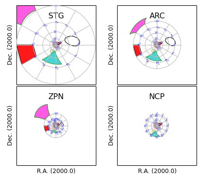
Note that some polygons could not be plotted for the NCP projection, simply because it is defined from declination 90 to 0 only. To avoid problems with divergence we limit the world coordinates to a declination of -30 degrees. The sky polygons are not aware of this limit and are plotted as long conversions between pixel- and world coordinates are possible. The ZPN example is a bit special. First, it is not possible to center a shape onto the pole (at least with the set of PV elements defined in the code) and second, we have a non zero PV2_0 element which breaks the relation between CRPIX and CRVAL.
For a detailed description of the input parameters of the used Skypolygon() method, read maputils.Annotatedimage.Skypolygon().
We arrived at a stage where one is challenged to apply different plot objects in one plot. Here is a practical example:
Example: mu_graticules.py - Combining plot with contours and a colorbar
1 2 3 4 5 6 7 8 9 10 11 12 13 14 15 16 17 18 19 20 21 22 23 24 25 26 27 28 29 30 31 32 33 34 35 36 37 38 39 40 41 42 43 44 45 46 47 | from kapteyn import maputils
from matplotlib import pyplot as plt
f = maputils.FITSimage("m101.fits")
f.set_limits(pxlim=(50,440), pylim=(50,450))
fig = plt.figure(figsize=(8,5.5))
frame = fig.add_axes((0.05, 0.1, 0.8, 0.7))
fig.text(0.5, 0.96, "Combination of plot objects",
horizontalalignment='center',
fontsize=14, color='r')
annim = f.Annotatedimage(frame, clipmin=3000, clipmax=15000)
cont = annim.Contours(levels=range(8000,14000,1000))
cont.setp_contour(linewidth=1)
cont.setp_contour(levels=11000, color='g', linewidth=2)
cb = annim.Colorbar(clines=True, orientation='vertical', fontsize=8, linewidths=5)
gr = annim.Graticule()
gr.setp_ticklabel(wcsaxis=0, fmt='HMS')
ilab = gr.Insidelabels(color='b', ha='left')
ilab.setp_label(position='14h03m0s', fontsize=15)
# Plot a second graticule for the galactic sky system
gr2 = annim.Graticule(deltax=7.5/60, deltay=5.0/60,
skyout="galactic",
visible=True)
gr2.setp_axislabel(plotaxis=("top","right"), label="Galactic l,b",
color='g', visible=True)
gr2.setp_axislabel(plotaxis=("left","bottom"), visible=False)
gr2.set_tickmode(plotaxis=("top","right"), mode="Native")
gr2.set_tickmode(plotaxis=("left","bottom"), mode="NO")
gr2.setp_ticklabel(wcsaxis=(0,1), color='g')
gr2.setp_ticklabel(plotaxis='right', fmt='DMs')
gr2.setp_tickmark(plotaxis='right', markersize=8, markeredgewidth=2)
gr2.setp_gratline(wcsaxis=(0,1), color='g')
annim.Ruler(x1=120, y1=100, x2=120, y2=330, step=1/60.0)
r1 = annim.Ruler(pos1='ga 102d0m, 59d50m', pos2='ga 102d7m30s, 59d50m',
world=True, step=1/60.0)
r1.setp_line(color='#ff22ff', lw=6)
r1.setp_label(color='m')
annim.Pixellabels(plotaxis='top', va='top')
pl = annim.Pixellabels(plotaxis='right')
pl.setp_marker(color='c', markersize=10)
pl.setp_label(color='m')
annim.plot()
plt.show()
|
(Source code, png, hires.png, pdf)

You are not restricted to FITS files to get plots of your data. The only requirement is that you must be able to get your data into a NumPy array and you need to supply a Python dictionary with FITS keywords. For both options we show an example.
Example: mu_externalheader.py - Header data from Python dictionary and setting a figure size
1 2 3 4 5 6 7 8 9 10 11 12 13 14 15 16 17 18 19 20 21 22 23 24 | from kapteyn import maputils
from matplotlib import pylab as plt
import numpy
header = {'NAXIS' : 2, 'NAXIS1': 800, 'NAXIS2': 800,
'CTYPE1' : 'RA---TAN',
'CRVAL1' :0.0, 'CRPIX1' : 1, 'CUNIT1' : 'deg', 'CDELT1' : -0.05,
'CTYPE2' : 'DEC--TAN',
'CRVAL2' : 0.0, 'CRPIX2' : 1, 'CUNIT2' : 'deg', 'CDELT2' : 0.05,
}
# Overrule the header value for pixel size in y direction
header['CDELT2'] = 0.3*abs(header['CDELT1'])
fitsobj = maputils.FITSimage(externalheader=header)
figsize = fitsobj.get_figsize(ysize=7, cm=True)
fig = plt.figure(figsize=figsize)
print "Figure size x, y in cm:", figsize[0]*2.54, figsize[1]*2.54
frame = fig.add_subplot(1,1,1)
mplim = fitsobj.Annotatedimage(frame)
gr = mplim.Graticule()
mplim.plot()
plt.show()
|
(Source code, png, hires.png, pdf)
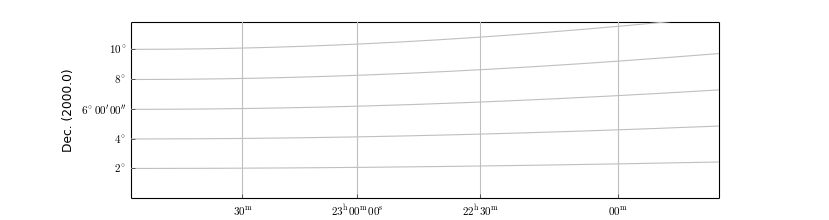
Example: mu_externaldata.py - Using external FITS header and data
1 2 3 4 5 6 7 8 9 10 11 12 13 14 15 16 17 18 19 20 21 22 23 24 25 26 27 28 29 30 31 32 33 | from kapteyn import maputils
from matplotlib import pylab as plt
import numpy
header = {'NAXIS' : 2, 'NAXIS1': 800, 'NAXIS2': 800,
'CTYPE1' : 'RA---TAN',
'CRVAL1' : 0.0, 'CRPIX1' : 1, 'CUNIT1' : 'deg', 'CDELT1' : -0.05,
'CTYPE2' : 'DEC--TAN',
'CRVAL2' : 0.0, 'CRPIX2' : 1, 'CUNIT2' : 'deg', 'CDELT2' : 0.05,
}
nx = header['NAXIS1']
ny = header['NAXIS2']
sizex1 = nx/2.0; sizex2 = nx - sizex1
sizey1 = nx/2.0; sizey2 = nx - sizey1
x, y = numpy.mgrid[-sizex1:sizex2, -sizey1:sizey2]
edata = numpy.exp(-(x**2/float(sizex1*10)+y**2/float(sizey1*10)))
f = maputils.FITSimage(externalheader=header, externaldata=edata)
f.writetofits()
fig = plt.figure(figsize=(6,5))
frame = fig.add_axes([0.1,0.1, 0.82,0.82])
mplim = f.Annotatedimage(frame, cmap='pink')
mplim.Image()
gr = mplim.Graticule()
gr.setp_gratline(color='y')
mplim.plot()
mplim.interact_toolbarinfo()
mplim.interact_imagecolors()
mplim.interact_writepos()
plt.show()
|
(Source code, png, hires.png, pdf)
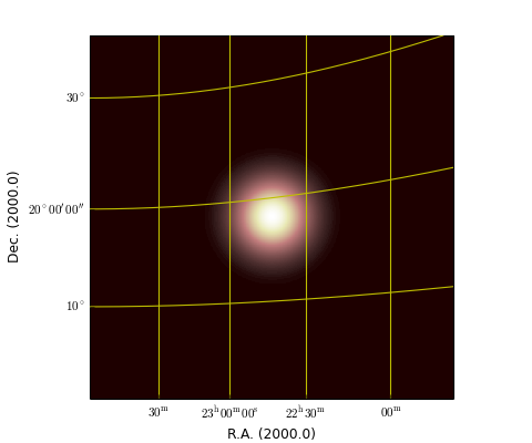
Note
Manipulated headers and data can be written to a FITS file with method maputils.FITSimage.writetofits(). Its documentation shows how to manipulate the format in which the data is written. Also have a look at this example which creates a FITSobject from an external header and external data. It then writes the object to a FITS file. The first time in the original data format with the original comments and history cards. The second time it writes to a file with BITPIX=-32 and it skips all comment and history information:
1 2 3 4 5 6 7 8 9 10 11 12 13 14 15 16 17 | from kapteyn import maputils
fitsobject = maputils.FITSimage(promptfie=maputils.prompt_fitsfile)
header = fitsobject.hdr
edata = fitsobject.dat
f = maputils.FITSimage(externalheader=header, externaldata=edata)
f.writetofits(history=True, comment=True,
bitpix=fitsobject.bitpix,
bzero=fitsobject.bzero,
bscale=fitsobject.bscale,
blank=fitsobject.blank)
f.writetofits("standard.fits", history=False, comment=False)
# or use parameter append to append to an existing file:
f.writetofits("existing.fits", append=True, history=False, comment=False)
|
We use the method with external headers also to create all sky maps. In the next example we demonstrate how a graticule is created for an all sky map. You will find examples about plotting data in these plots in the document about all sky maps.
Example: mu_allsky_single.py - Using Python dictionary to define all-sky map
1 2 3 4 5 6 7 8 9 10 11 12 13 14 15 16 17 18 19 20 21 22 23 24 25 26 27 28 29 30 31 32 33 34 35 36 37 38 39 40 41 | from kapteyn import maputils
from numpy import arange
from matplotlib import pyplot as plt
dec0 = 89.9999999999 # Avoid plotting on the wrong side
header = {'NAXIS' : 2,
'NAXIS1' : 100, 'NAXIS2': 80,
'CTYPE1' : 'RA---TAN',
'CRVAL1' : 0.0, 'CRPIX1' : 50, 'CUNIT1' : 'deg',
'CDELT1' : -5.0, 'CTYPE2' : 'DEC--TAN',
'CRVAL2' : dec0, 'CRPIX2' : 40,
'CUNIT2' : 'deg', 'CDELT2' : 5.0,
}
X = arange(0,360.0,15.0)
Y = [20, 30,45, 60, 75, 90]
fig = plt.figure(figsize=(7,6))
frame = fig.add_axes((0.1,0.1,0.8,0.8))
f = maputils.FITSimage(externalheader=header)
annim = f.Annotatedimage(frame)
grat = annim.Graticule(wylim=(20.0,90.0), wxlim=(0,360), startx=X, starty=Y)
lon_world = range(0,360,30)
lat_world = [20, 30, 60, dec0]
grat.setp_gratline(position=20, color='g', linestyle='--')
# Plot labels inside the plot
lon_constval = None
lat_constval = 18
il1 = grat.Insidelabels(wcsaxis=0,
world=lon_world, constval=lat_constval, fmt='Dms')
il1.setp_label(color='r', fontsize=15)
il2 = grat.Insidelabels(wcsaxis=1, deltapy=2,
world=lat_world, constval=lon_constval, fmt='Dms')
il2.setp_label(color='b', fontsize=10)
annim.plot()
# Set title for Matplotlib
title = r"Gnomonic projection (TAN) diverges at $\theta=0$. (Cal. fig.8)"
frame.set_title(title, color='g', y=1.02)
plt.show()
|
(Source code, png, hires.png, pdf)

The data from a FITS file is stored in a NumPy array. Then it is straightforward to maniplate this data. NumPy has many methods for this. We apply a Fourier transform to an image of M101. We show how to use functions abs and angle with a complex array as argument to get images of the amplitude and the fase of the transform. With the transform we test the inverse procedure and show the residual. There seems to be some systematic structure in the residual map but notice that the maximum is very small compared to the smallest image value in the original (which is around 1500). We used NumPy’s FFT functions to calculate the transform. Have a look at the code:
Example: mu_fft.py - Mosaic of plots showing FFT of image data and inverse transform
1 2 3 4 5 6 7 8 9 10 11 12 13 14 15 16 17 18 19 20 21 22 23 24 25 26 27 28 29 30 31 32 33 34 35 36 37 38 39 40 41 42 43 44 45 46 47 48 49 50 51 52 53 54 55 56 57 58 | from kapteyn import maputils
from matplotlib import pyplot as plt
from numpy import fft, log, abs, angle
f = maputils.FITSimage("m101.fits")
yshift = -0.1
fig = plt.figure(figsize=(8,6))
fig.subplots_adjust(left=0.01, bottom=0.1, right=1.0, top=0.98,
wspace=0.03, hspace=0.16)
frame = fig.add_subplot(2,3,1)
frame.text(0.5, yshift, "M101", ha='center', va='center',
transform = frame.transAxes)
mplim = f.Annotatedimage(frame, cmap="spectral")
mplim.Image()
fftA = fft.rfft2(f.dat, f.dat.shape)
frame = fig.add_subplot(2,3,2)
frame.text(0.5, yshift, "Amplitude of FFT", ha='center', va='center',
transform = frame.transAxes)
f = maputils.FITSimage("m101.fits", externaldata=log(abs(fftA)+1.0))
mplim2 = f.Annotatedimage(frame, cmap="gray")
im = mplim2.Image()
frame = fig.add_subplot(2,3,3)
frame.text(0.5, yshift, "Phase of FFT", ha='center', va='center',
transform = frame.transAxes)
f = maputils.FITSimage("m101.fits", externaldata=angle(fftA))
mplim3 = f.Annotatedimage(frame, cmap="gray")
im = mplim3.Image()
frame = fig.add_subplot(2,3,4)
frame.text(0.5, yshift, "Inverse FFT", ha='center', va='center',
transform = frame.transAxes)
D = fft.irfft2(fftA)
f = maputils.FITSimage("m101.fits", externaldata=D.real)
mplim4 = f.Annotatedimage(frame, cmap="spectral")
im = mplim4.Image()
frame = fig.add_subplot(2,3,5)
Diff = D.real - mplim.data
f = maputils.FITSimage("m101.fits", externaldata=Diff)
mplim5 = f.Annotatedimage(frame, cmap="spectral")
im = mplim5.Image()
frame.text(0.5, yshift, "M101 - inv. FFT", ha='center', va='center',
transform = frame.transAxes)
s = "Residual with min=%.1g max=%.1g" % (Diff.min(), Diff.max())
frame.text(0.5, yshift-0.08, s, ha='center', va='center',
transform = frame.transAxes, fontsize=8)
mplim.interact_imagecolors()
mplim2.interact_imagecolors()
mplim3.interact_imagecolors()
mplim4.interact_imagecolors()
mplim5.interact_imagecolors()
maputils.showall()
|
(Source code, png, hires.png, pdf)

Fig. mu_fft.py - FFT: another use of external data
The example shows that we can use external data with the correct shape in combination with the original FITS header. Note that we used Matplotlib’s text() method instead of xlabel(). The reason is that the primary frame has all its axes set to invisible. We can set them to visible but besides a label, one also get numbers along the axes and that was what we want to avoid.
There are several methods to compare data of the same part of the sky but from different sources. These different sources often have different world coordinate systems. If you want to compare two or more sources in one plot you need to define a base world coordinate system (wcs) and adjust the other sources so that their data fits the header description of the first. In other words: you need to re-project the data of the other sources. Module wcs provides a powerful coordinate transformation function called wcs.coordmap() which does the necessary coordinate transformations between two wcs systems. The transformation of the data is done with an interpolation function based Scipy’s function map_coordinates. The two functions are combined in method maputils.FITSimage.reproject_to(). If you have a FITS data structure that contains more than one spatial map (in the same hdu), then the method will re-project all these maps to a new spatial structure given in a second FITSimage object. This is demonstrated in the next example
Example: mu_reproj.py - Use second FITSimage object to define re-projection
1 2 3 4 5 6 7 8 9 10 11 12 13 14 15 16 17 18 | from kapteyn import maputils
# Read first image as base
Basefits = maputils.FITSimage("ra_pol_freq_dec.fits")
# Get data from a FITS file. This is the data that
# should be reprojected to fit the header of Basefits.
Secondfits = maputils.FITSimage("dec_pol_freq_ra.fits")
# Now we want to re-project the data of the Base object onto
# the wcs of the second object. This is done with the
# reproject_to() method of the first FITSimage object
# (the data object) with the header of the second FITSimage
# object as parameter. This results in a new FITSimage object
Reprojfits = Basefits.reproject_to(Secondfits.hdr)
# Write the result to disk
Reprojfits.writetofits("reproj.fits", clobber=True)
|
Note that the result has the same structure for all non spatial axes, while the spatial information is copied from the second object.
If you want only a selection of all the available spatial maps, then you can restrict the re-projection with parameters plimlo and plimhi. These parameters are single pixel coordinates or tuples with pixel coordinates and each pixel coordinate represents a position on a non-spatial axis (a repeat axis) similar to the definition of a slice. Also it is possible to set the pixel limits of the output spatial structure with pxlim and pylim. Note that these correspond to the axis order of the spatial map to which we want to re-project. With these parameters it is easy to extend a map e.g. so that it contains a rotated map without cutting the edges. For all these procedures, the appropriate values of CRPIX in the header are adjusted so that the output header describes a valid wcs.
Below we show how to decrease the output size for the spatial axes. Also we require two maps in the output: the first is at POL=1 and FREQ=7 and the second is at POL=1 and FREQ=8. Note that plimlo and plimhi describe contiguous ranges!
>>> Reprojfits = Basefits.reproject_to(Secondfits.hdr,
                                       pxlim=(3,30), pylim=(3,20),
                                       plimlo=(1,7), plimhi=(1,8))
You can also expand the output for the spatial maps by entering values outside the default ranges [1, NAXIS]. Negative values are allowed to expand beyond pixel coordinate 1. The next code fragment shows this for all spatial maps at POL=1 (i.e. for all pixels coordinates on the FREQ axis).
>>> Reprojfits = Basefits.reproject_to(Secondfits.hdr,
                                       pxlim=(-10,50), pylim=(-10,50),
                                       plimlo=1, plimhi=1)
As an alternative to re-projecting to an existing header of a different wcs, one can also make a copy of a header and adjust it by making changes to existing keywords or to add new keyword, value pairs. This is one of the more common applications for re-projection purposes. For instance, one can change the header value for CROTA (corresponding to the latitude axis of an image) to rotate a map. Or one can re-project to another projection e.g. from a Gnomonic projection (TAN) to a Mercator projection (MER). This is what we have done in the next script. In the familiar M101 FITS file, we increased the pixel sizes with a factor of 100 to demonstrate the effect of the re-projection.
There are two practical problems we have to address:
- The CRVAL’s for a Mercator projection must be 0.0. If we don’t change them, the projection will be oblique.
- We don’t know how big the result must be (in terms of pixels) to fit the result.
These problems are solved by creating an intermediate FITSimage object with the new header where CRVAL is set to 0 and where the values of CTYPE were changed. Then the pixel positions of the border of the original image are used to find world coordinates in the original image and from these world coordinates we derive pixel coordinates in the new projection. From these positions we take the minimum and maximum to extend the output box so that it can hold the entire image without any clipping.
We end up with the rectangular system that we are used to from a Mercator projection. Note that the image is subject to a small rotation.
Example: mu_m1012mercator.py - Transforming a map to another projection
1 2 3 4 5 6 7 8 9 10 11 12 13 14 15 16 17 18 19 20 21 22 23 24 25 26 27 28 29 30 31 32 33 34 35 36 37 38 39 40 41 42 | from kapteyn import maputils
from matplotlib import pyplot as plt
import numpy as np
Basefits = maputils.FITSimage("m101big.fits")
hdr = Basefits.hdr.copy()
hdr['CTYPE1'] = 'RA---MER'
hdr['CTYPE2'] = 'DEC--MER'
hdr['CRVAL1'] = 0.0
hdr['CRVAL2'] = 0.0
naxis1 = Basefits.hdr['NAXIS1']
naxis2 = Basefits.hdr['NAXIS2']
# Sample the border in pixels
x = np.concatenate([np.arange(1, naxis1+1), naxis1*np.ones(naxis1),
np.arange(1, naxis1+1), np.ones(naxis1)])
y = np.concatenate([np.ones(naxis2), np.arange(1, naxis2+1),
naxis2*np.ones(naxis1), np.arange(1, naxis2+1)])
x, y = Basefits.proj.toworld((x,y))
# Create a dummy object to calculate pixel coordinates of border in the new system.
f = maputils.FITSimage(externalheader=hdr)
px, py = f.proj.topixel((x,y))
pxlim = [int(min(px))-1, int(max(px))+1]
pylim = [int(min(py))-1, int(max(py))+1]
# print "New limits:", pxlim, pylim
Reprojfits = Basefits.reproject_to(hdr, pxlim_dst=pxlim, pylim_dst=pylim)
#Reprojfits.writetofits("reproj.fits", clobber=True)
fig = plt.figure(figsize=(9,5))
frame1 = fig.add_subplot(1,2,1)
frame2 = fig.add_subplot(1,2,2)
im1 = Basefits.Annotatedimage(frame1)
im2 = Reprojfits.Annotatedimage(frame2)
im1.Image(); im1.Graticule()
im2.Image(); im2.Graticule()
im1.plot(); im2.plot()
fig.tight_layout()
plt.show()
|
(Source code, png, hires.png, pdf)

In the previous section we have dealt with a change in the projection only and we needed to set explicit values for CRVAL. But what if we want to change both projection system and sky system. For example, we want to transform our M101 FITS file to a map with a Galactic sky system and we want to change the projection type from TAN to SIN. Now we need an extra step to find the values for CRVAL in the galactic system that correspond to the values of CRVAL in the original file. We do this with class wcs.Transformation which transforms world coordinates from one celestial system to the other.
We apply the same trick with the border pixels, but now we need to convert the world coordinates of the border to world coordinates in the Galactic system.
Example: mu_skyAndProj.py - Transforming a map to another projection AND another sky system
1 2 3 4 5 6 7 8 9 10 11 12 13 14 15 16 17 18 19 20 21 22 23 24 25 26 27 28 29 30 31 32 33 34 35 36 37 38 39 40 41 42 43 44 45 46 47 48 49 50 51 52 53 54 55 56 57 58 59 60 61 62 | from kapteyn import maputils, wcs
from matplotlib import pyplot as plt
import numpy as np
# The data you want to re-project
Basefits = maputils.FITSimage("m101.fits")
hdrIn = Basefits.hdr
projIn = Basefits.proj
crvalsI = Basefits.proj.crval
# We want to change the sky system, so we need to know the values of CRVAL in the new system
trans = wcs.Transformation(projIn.skysys, skyout=wcs.galactic)
crvalsO = trans(crvalsI)
# Adjust the new header which was derived from the input
hdrOut = hdrIn.copy()
hdrOut['CTYPE1'] = 'GLON-SIN'
hdrOut['CTYPE2'] = 'GLAT-SIN'
hdrOut['CRVAL1'] = crvalsO[0]
hdrOut['CRVAL2'] = crvalsO[1]
# Get an estimate of the new corners by converting ALL boundary pixels of the input map
naxis1 = hdrIn['NAXIS1']
naxis2 = hdrIn['NAXIS2']
x = np.concatenate([np.arange(1, naxis1+1), naxis1*np.ones(naxis1),
np.arange(1, naxis1+1), np.ones(naxis1)])
y = np.concatenate([np.ones(naxis2), np.arange(1, naxis2+1),
naxis2*np.ones(naxis1), np.arange(1, naxis2+1)])
x, y = projIn.toworld((x,y))
# But we need Galactic coordinates before converting to pixels
# in the new system, not the original cooordinates:
x, y = trans((x,y))
# Create a dummy object to calculate pixel coordinates in the new system.
f = maputils.FITSimage(externalheader=hdrOut)
px, py = f.proj.topixel((x,y))
pxlim = [int(min(px))-1, int(max(px))+1]
pylim = [int(min(py))-1, int(max(py))+1]
#print "New limits:", pxlim, pylim
# Do the re-projection
Reprojfits = Basefits.reproject_to(hdrOut, pxlim_dst=pxlim, pylim_dst=pylim)
#Reprojfits.writetofits("reproj.fits", clobber=True)
crpixs = Reprojfits.proj.crpix
crvals = Reprojfits.proj.toworld(crpixs)
#print "Check that crpix values in output are adjusted correctly:"
#print "Crvals from initial transformation and from re-projection:", crvals, crvalsO
# Some plotting to check the result
fig = plt.figure(figsize=(9,5))
frame1 = fig.add_subplot(1,2,1)
frame2 = fig.add_subplot(1,2,2)
im1 = Basefits.Annotatedimage(frame1)
im2 = Reprojfits.Annotatedimage(frame2)
im1.Image(); im1.Graticule()
im2.Image(); im2.Graticule()
im1.interact_toolbarinfo()
im2.interact_toolbarinfo()
im1.plot(); im2.plot()
fig.tight_layout()
plt.show()
|
(Source code, png, hires.png, pdf)

To facilitate legacy FITS readers which cannot process CD and PC elements we wrote a method that converts headers to classic headers, i.e. with the familiar header keywords CRVAL, CRPIX, CDELT, CROTA. When a CD or PC matrix is encountered, and the non diagonal elements are not zero, then skew can be expected. One derives then two values for the image rotation. This method averages these values as a ‘best value’ for CROTA. (see also section 6 in paper II by Calabretta & Greisen).
Example: mu_reproj2classic.py - Create a ‘classic’ header without CD or PC elements
1 2 3 4 5 6 7 8 9 10 11 12 13 14 15 16 17 18 19 20 21 22 23 24 25 26 27 28 29 30 31 32 33 34 35 36 37 38 39 40 41 42 | from kapteyn import maputils, wcs
from math import * # To support expression evaluation with 'eval()'
Basefits = maputils.FITSimage(promptfie=maputils.prompt_fitsfile)
classicheader, skew, hdrchanged = Basefits.header2classic()
if hdrchanged:
print "Original header:\n", Basefits.str_header()
if skew != 0.0:
print "Found two different rotation angles. Difference is %f deg." % skew
else:
print "Header probably already 'classic'. Nothing changed"
print """You can copy the data and replace the header by the classic header
or you can re-project it to get rid of skew or to rotate the data
using a rotation angle (keyword CROTAn=)."""
ok = raw_input("Do you want to remove skew or rotate image ... [Y]/N: ")
if ok in ['y', 'Y', '']:
lat = Basefits.proj.lataxnum
key = "CROTA%d"%lat
crotaold = classicheader[key] # CROTA Is always available in this header
mes = "Enter value for CROTA%d ... [%g]: " %(lat, crotaold)
newcrota = raw_input(mes)
if newcrota != '':
crota = eval(newcrota)
classicheader[key] = crota
print "Classic header voor reproject:"
print classicheader
print "\n Re-projecting ..."
fnew = Basefits.reproject_to(classicheader, insertspatial=False)
else:
# A user wants to replace the header only. Leave data untouched.
fnew = maputils.FITSimage(externalheader=classicheader,
externaldata=Basefits.dat)
filename_out = "classic.fits"
# ADD (!) to 'classic.fits'
print "A copy of the selected hdu in the FITS file is APPENDED to [%s] on disk"%filename_out
fnew.writetofits(filename_out, clobber=True, append=True)
|
Method maputils.FITSimage.reproject_to() recognizes three input types for parameter reprojobj. We demonstrated the use of a FITSimage object and a header. It is also possible to set its value to None. Then the header of the current object is used to define the transformation. If you don’t want to get the header and change it in your script (as in a previous example) then one can use keyword parameters with the same name as FITS keywords to change this current header. In the next example we show how to rotate an image using the rotation parameter and increase the size of the image using keyword parameters. It also shows a hint how to align an image with the direction of the north, which combines the use of parameter rotation to create a header for which CROTAn defines the rotation of the image and keyword CROTA2 to set this header value to 0.0.
Example: mu_simplereproj.py - Rotate an image using keyword parameters
1 2 3 4 5 6 7 8 9 10 11 12 13 14 15 16 17 | from kapteyn import maputils
Basefits = maputils.FITSimage(promptfie=maputils.prompt_fitsfile)
Rotfits = Basefits.reproject_to(rotation=40.0, naxis1=800, naxis2=800,
crpix1=400, crpix2=400)
# If you want alignment with direction of the north, use:
# Rotfits = Basefits.reproject_to(rotation=0.0, crota2=0.0)
# If copy on disk required:
# Rotfits.writetofits("aligned.fits", clobber=True, append=False)
annim = Rotfits.Annotatedimage()
annim.Image()
annim.Graticule()
annim.interact_toolbarinfo()
maputils.showall()
|
Re-projections are often used to enable the comparison of data of two different sources (i.e. with different world coordinate systems) in one plot. Then usually contours of a second FITS image are used upon an image of a base FITS image. The situation is a bit different compared to the examples above. We need only one spatial map to be re-projected and this spatial map is set by a slice (i.e. pixel positions on the repeat axes). The pixel limits (box) of the spatial axes are set by the first FITS image. Instead of a header we can use the FITSimage object to which we want to re-project as a parameter. Then all appropriate information is passed and the maputils.FITSimage.reproject_to() method returns a new FITSimage object with only one spatial map with sizes that fits the first spatial map. The attribute boxdat can be used to replace the contents of the first image using the boxdat parameter in method maputils.FITSimage.Annotatedimage().
The example script below shows how this is implemented in a script. The situation is not very complicated because we deal with two 2-dimensional data structures. Note the use of histogram equalization to enhance some details.
Example: mu_overlayscuba.py - Overlay image with different world coordinate system
1 2 3 4 5 6 7 8 9 10 11 12 13 14 15 16 17 18 19 20 21 22 23 24 25 26 27 28 29 | from kapteyn import maputils
from matplotlib import pyplot as plt
file1 = "scuba850_AFGL2591.fits"
file2 = "13CO_3-2_integ_regrid.fits"
# Read first image as base
Basefits = maputils.FITSimage(file1)
Secondfits = maputils.FITSimage(file2)
Reprojfits = Secondfits.reproject_to(Basefits)
fig = plt.figure()
frame = fig.add_subplot(1,1,1)
baseim = Basefits.Annotatedimage(frame)
baseim.Image()
baseim.set_histogrameq()
baseim.Graticule()
overlayim = Basefits.Annotatedimage(frame, boxdat=Reprojfits.boxdat)
levels = range(20,200,20)
overlayim.Contours(levels=levels, colors='w')
baseim.plot()
overlayim.plot()
baseim.interact_toolbarinfo()
baseim.interact_imagecolors()
plt.show()
|
(Source code, png, hires.png, pdf)

It is also possible to mix two images using an alpha factor smaller than 1.0. That is what we did in the next example. The overlay image is smaller than the base image. Then the overlay is padded with NaN’s which are not transparent. We can change the values for pixels that could not be interpolated from NaN to another value with parameter cval which is part of a dictionary with keywords and values to control the interpolation routine in maputils.FITSimage.reproject_to(). We also set the interpolation order to 1 (which is the default set by maputils). This order represents a bilinear interpolation.
Example: mu_overlayscuba_im.py - Overlay image with different world coordinate system, using transparancy factor
1 2 3 4 5 6 7 8 9 10 11 12 13 14 15 16 17 18 19 20 21 22 23 24 25 26 27 28 29 30 31 32 33 34 35 | from kapteyn import maputils
from matplotlib import pyplot as plt
file1 = "scuba850_AFGL2591.fits"
file2 = "13CO_3-2_integ_regrid.fits"
# Read first image as base
Basefits = maputils.FITSimage(file1)
Secondfits = maputils.FITSimage(file2)
pars = dict(cval=0.0, order=1)
Reprojfits = Secondfits.reproject_to(Basefits, interpol_dict=pars)
fig = plt.figure()
frame = fig.add_subplot(1,1,1)
baseim = Basefits.Annotatedimage(frame)
baseim.Image(alpha=1.0)
baseim.set_histogrameq()
baseim.set_blankcolor('k')
baseim.Graticule()
overlayim = Basefits.Annotatedimage(frame, cmap='OrRd',
boxdat=Reprojfits.boxdat)
levels = range(50,200,20)
#overlayim.Contours(levels=levels, colors='w')
overlayim.Image(alpha=0.8)
baseim.set_histogrameq()
baseim.plot()
overlayim.plot()
baseim.interact_toolbarinfo()
baseim.interact_imagecolors()
plt.show()
|
(Source code, png, hires.png, pdf)
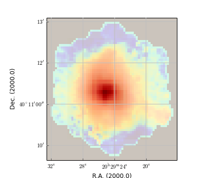
The base image has scheduled a function to interactively change its colors while the second image remains fixed. This enables you do compare the two images.
We like to add an example where we combine an all-sky image with an all-sky graticule. If your goal is to plot an all-sky image with a graticules overlay then you have to use the method that plots labels inside the image area to get the best results. This method is from class Annotatedimage and is called Insidelabels(), see description at: wcsgrat.Graticule.Insidelabels()
But your mission is not always straightforward as it seems. For instance, when you want to plot a map in a different sky system and/or projection system, you need to re-project the image first. Here we present an example where we start with an all-sky map in galactic coordinates but without a projection system defined in its header. We want to show the data in an oblique Aitof projection.
First obtain an all sky map. This is what we have done for our example: Go to the Bonn 408-MHz All-Sky Survey
You need to enter information on a form. First, there is no need to enter coordinates for the center. For the map size in x and y take 360 180 (degrees), i.e. the whole sky For the tabular interval, take the original values (i.e. enter -1 -1) Select Galactic coordinates as the sky system and pixmap (no projection) as the projection system. In ‘Select a survey’ we selected ‘All sky 408 Mhz’. Submit form and wait for the map to appear. Then download the FITS file (one of the buttons below the image).
In the script we change this FITS file’s CTYPE’s to ‘GLON-CAR’ and ‘GLAT-CAR’. WCS projection CAR is a valid WCSLIB rectangular projection. We can do this safely because the values of CRVAL are 0.0 and they represent the center of the image (CRPIX=NAXIS/2). So the standard parallel is the equator. Now the previously linear projection has a WCS equivalent and we can use it for our reprojections. If you wonder why we needed to apply this trick, then you should try the example without adding the projection type ‘CAR’. You will end up with only one half of the entire sky. The reason is that we sample the output in pixels. These pixels are converted into world coordinates of the output image. But these world coordinates are between 0 and 360 degrees in longitude. If you enter these coordinates in the linear system, you get pixels outside the range of pixels for the input set because there the range in longitude is between -180 and 180 degrees (CRVAL’s are in the center) and a linear system does not wrap around.
Example: mu_allsky_reproj.py - Reproject all-sky map to fit graticules of self defined projection system
1 2 3 4 5 6 7 8 9 10 11 12 13 14 15 16 17 18 19 20 21 22 23 24 25 26 27 28 29 30 31 32 33 34 35 36 37 38 39 40 41 42 43 44 45 46 47 48 49 50 51 52 53 54 55 56 57 58 59 60 61 62 63 64 65 66 67 68 69 70 71 72 73 74 75 76 77 78 79 80 81 82 83 84 85 86 87 88 89 90 91 92 93 94 95 96 97 98 99 100 101 102 103 104 | import numpy
from kapteyn import maputils
from matplotlib.pyplot import show, figure
import csv # Read some poitions from file in Comma Separated Values format
# Some initializations
blankcol = "#334455" # Represent undefined values by this color
epsilon = 0.0000000001
figsize = (9,7) # Figure size in inches
plotbox = (0.1,0.05,0.8,0.8)
fig = figure(figsize=figsize)
frame = fig.add_axes(plotbox)
Basefits = maputils.FITSimage("allsky_raw.fits") # Here is your downloaded FITS file in rectangular coordinates
Basefits.hdr['CTYPE1'] = 'GLON-CAR' # For transformations we need to give it a projection type
Basefits.hdr['CTYPE2'] = 'GLAT-CAR' # CAR is rectangular
# Use some header values to define reprojection parameters
cdelt1 = Basefits.hdr['CDELT1']
cdelt2 = Basefits.hdr['CDELT2']
naxis1 = Basefits.hdr['NAXIS1']
naxis2 = Basefits.hdr['NAXIS2']
# Header works only with a patched wcslib 4.3
# Note that changing CRVAL1 to 180 degerees, shifts the plot 180 deg.
header = {'NAXIS' : 2, 'NAXIS1': naxis1, 'NAXIS2': naxis2,
'CTYPE1' : 'GLON-AIT',
'CRVAL1' : 0, 'CRPIX1' : naxis1//2, 'CUNIT1' : 'deg', 'CDELT1' : cdelt1,
'CTYPE2' : 'GLAT-AIT',
'CRVAL2' : 30.0, 'CRPIX2' : naxis2//2, 'CUNIT2' : 'deg', 'CDELT2' : cdelt2,
'LONPOLE' :60.0,
'PV1_1' : 0.0, 'PV1_2' : 90.0, # IMPORTANT. This is a setting from Cal.section 7.1, p 1103
}
Reprojfits = Basefits.reproject_to(header)
annim_rep = Reprojfits.Annotatedimage(frame)
annim_rep.set_colormap("heat.lut") # Set color map before creating Image object
annim_rep.set_blankcolor(blankcol) # Background are NaN's (blanks). Set color here
annim_rep.Image(vmin=30000, vmax=150000) # Just a selection of two clip levels
annim_rep.plot()
# Draw the graticule, but do not cover near -90 to prevent ambiguity
X = numpy.arange(0,390.0,15.0);
Y = numpy.arange(-75,90,15.0)
f = maputils.FITSimage(externalheader=header)
annim = f.Annotatedimage(frame)
grat = annim.Graticule(axnum= (1,2), wylim=(-90,90.0), wxlim=(0,360),
startx=X, starty=Y)
grat.setp_lineswcs0(0, color='w', lw=2)
grat.setp_lineswcs1(0, color='w', lw=2)
# Draw border with standard graticule, just to make the borders look smooth
header['CRVAL1'] = 0.0
header['CRVAL2'] = 0.0
del header['PV1_1']
del header['PV1_2']
header['LONPOLE'] = 0.0
header['LATPOLE'] = 0.0
border = annim.Graticule(header, axnum= (1,2), wylim=(-90,90.0), wxlim=(-180,180),
startx=(180-epsilon, -180+epsilon), skipy=True)
border.setp_lineswcs0(color='w', lw=2) # Show borders in arbitrary color (e.g. background color)
border.setp_lineswcs1(color='w', lw=2)
# Plot the 'inside' graticules
lon_constval = 0.0
lat_constval = 0.0
lon_fmt = 'Dms'; lat_fmt = 'Dms' # Only Degrees must be plotted
addangle0 = addangle1=0.0
deltapx0 = deltapx1 = 1.0
labkwargs0 = {'color':'r', 'va':'center', 'ha':'center'}
labkwargs1 = {'color':'r', 'va':'center', 'ha':'center'}
lon_world = range(0,360,30)
lat_world = [-60, -30, 30, 60]
ilabs1 = grat.Insidelabels(wcsaxis=0,
world=lon_world, constval=lat_constval,
deltapx=1.0, deltapy=1.0,
addangle=addangle0, fmt=lon_fmt, **labkwargs0)
ilabs2 = grat.Insidelabels(wcsaxis=1,
world=lat_world, constval=lon_constval,
deltapx=1.0, deltapy=1.0,
addangle=addangle1, fmt=lat_fmt, **labkwargs1)
# Read marker positions (in 0h0m0s 0d0m0s format) from file
reader = csv.reader(open("positions.txt"), delimiter=' ', skipinitialspace=True)
for line in reader:
if line:
hms, dms = line
postxt = "{eq fk4-no-e} "+hms+" {} "+dms # Define the sky system of the source
print postxt
annim.Marker(pos=postxt, marker='*', color='yellow', ms=20)
# Plot a title
titlepos = 1.02
title = r"""All sky map in Hammer Aitoff projection (AIT) oblique with:
$(\alpha_p,\delta_p) = (0^\circ,30^\circ)$, $\phi_p = 75^\circ$ also:
$(\phi_0,\theta_0) = (0^\circ,90^\circ)$."""
t = frame.set_title(title, color='g', fontsize=13, linespacing=1.5)
t.set_y(titlepos)
annim.plot()
annim.interact_toolbarinfo()
annim_rep.interact_imagecolors()
show()
|
(Source code, png, hires.png, pdf)
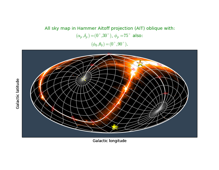
In the plot we marked some positions with a yellow star. The method that we use here to read positions from a file is different compared to previous examples. That is because we have a file where the positions are represented by strings. So we implemented some code to read these positions. The positions must follow the syntax for positions as described in: Module positions. The contents of the text file with some marker positions is:
17h45m40.0409s   -29d0m28.118s
12h49m0s         27d24m
17h42m37s        -28d57m0s
3h10m07s  20d10m0s
3h11m07s  21d10m0s
3h12m07s  22d10m0s
3h13m07s  23d10m0s
3h14m07s  24d10m0s
3h15m07s  25d10m0s
As you can see, the positions are equatorial. But there is no way for the program to detect which sky- and reference system is used for the positions. Therefore we iterate over all position strings and add the right specification. In our example this is {eq fk4-no-e}.
The interpolation routine in the Kapteyn Package is based on SciPy’s map_coordinates(). This function has a parameter order which sets the interpolation mode. In the script below we create a contour overlay using a rotated version of a base image (also the pixel size differs). This version is re-projected onto the first. The difference map is used to calculate a mean and a standard deviation of the residual. In a table we show the calculated values as function of the interpolation order:
| order | interpolation | mean | std | sum |
|---|---|---|---|---|
| 0 | Nearest int | 0.174 | 194 | 35337 |
| 1 | Linear | 0.067 | 156 | 13728 |
| 2 | Quadratic | 0.034 | 113 | 6821 |
| 3 | Spline order 3 | 0.032 | 111 | 6430 |
| 4 | order 4 | 0.031 | 108 | 6238 |
| 5 | order 5 | 0.030 | 107 | 6183 |
So order=2 or order=3 seems a reasonable choice.
If you zoom the third figure, you will see that the red contours closely follow the green contours that were drawn first. This is also a measure of the precision in the re-projection because the intensities in the two images are the same.
Example: mu_overlaym101.py - Re-projection test with overlay data
1 2 3 4 5 6 7 8 9 10 11 12 13 14 15 16 17 18 19 20 21 22 23 24 25 26 27 28 29 30 31 32 33 34 35 36 37 38 39 40 41 42 43 44 45 46 47 48 49 50 51 52 53 54 55 56 57 58 59 60 61 62 63 64 65 66 67 68 69 70 | from kapteyn import maputils
from matplotlib import pyplot as plt
import numpy
#order = input("Enter order of spline interpolation in range 0..5: ")
order = 1
if order < 0: order = 0
if order > 5: order = 5
file1 = "m101OPT.fits"
Basefits = maputils.FITSimage(file1)
pxlim = (50,500); pylim = (50,500)
Basefits.set_limits(pxlim, pylim)
file2 = "m101HI.fits"
Overfits = maputils.FITSimage(file2)
Overfits.set_imageaxes(1,2)
# Not necessary to set limits if an overlay is required
fig = plt.figure(figsize=(6,7))
frame1 = fig.add_subplot(2,2,1)
frame2 = fig.add_subplot(2,2,2)
frame3 = fig.add_subplot(2,2,3)
frame4 = fig.add_subplot(2,2,4)
fs = 10 # Font size for titles
levels = [8000, 12000]
# Plot 1: Base
baseim = Basefits.Annotatedimage(frame1)
baseim.Image()
frame1.set_title("WCS1", fontsize=fs)
# Plot 2: Data with different wcs
overlayim = Overfits.Annotatedimage(frame2)
overlayim.Image()
overlayim.set_blankcolor('y')
frame2.set_title("WCS2", fontsize=fs)
# Plot 3: Base with contours reprojected from other source
baseim2 = Basefits.Annotatedimage(frame3)
baseim2.Image()
baseim2.Contours(levels=levels, colors='g')
# Filter the NaN's. Replace by 0.0 to be able tu use spline order > 1
#Overfits.boxdat[numpy.where(numpy.isnan(Overfits.boxdat))] = 0.0
# Set parameters for the interpolation routine
pars = dict(cval=numpy.nan, order=order)
Reprojfits = Overfits.reproject_to(Basefits, interpol_dict=pars)
overlayim2 = Basefits.Annotatedimage(frame3, boxdat=Reprojfits.boxdat)
overlayim2.Contours(levels=levels, colors='r')
frame3.set_title("Image WCS1 + \ncontours reprojected WCS2", fontsize=fs)
# Plot 4: Plot the difference between base and reprojection
x = Basefits.boxdat - overlayim2.data
print "Residual min, max, mean, std, sum:", x.flatten().min(), x.flatten().max(),\
x.flatten().mean(), x.flatten().std(), x.flatten().sum()
diff = Basefits.Annotatedimage(frame4, boxdat=x)
diff.Image()
diff.set_histogrameq()
frame4.set_title(r"$\Delta$ = WCS1 - reprojected WCS2", fontsize=fs)
# User interaction
diff.interact_toolbarinfo()
diff.interact_imagecolors()
overlayim.interact_imagecolors()
maputils.showall()
|
(Source code, png, hires.png, pdf)

There are many situations where you want to identify features using markers at positions listed in a file. These positions are world coordinates. and assumed to be in degrees. The format of the file we used to read positions is as follows:
segment 1  rank 4  points 169
      31.270000 32.268889
      31.148611 32.277500
      31.104722 32.171389
      31.061111 32.114444
      31.120833 32.056667
The first line is an example of a comment. Therefore we use in maputils.Annotatedimage.positionsfromfile() character ‘s’ as indentifier of a line with comments. In this method, the numbers are read from file with a method from module tabarray and are transformed to pixel coordinates in the projection system of the image in the FITS file. We changed the header values of CDELT a bit to get a bigger area in world coordinates. The positions are plotted as small dots. The dots represent coastlines in the Caribbean.
Example: mu_markersfromfile.py - Use special method to read positions from file and mark those positions
1 2 3 4 5 6 7 8 9 10 11 12 13 14 15 16 17 18 19 20 21 22 23 24 25 26 27 28 29 | from kapteyn import maputils
from matplotlib import pyplot as plt
from kapteyn import tabarray
import numpy
# Get a header and change some values
f = maputils.FITSimage("m101.fits")
header = f.hdr
header['CDELT1'] = 0.1
header['CDELT2'] = 0.1
header['CRVAL1'] = 285
header['CRVAL2'] = 20
# Use the changed header as external source for new object
f = maputils.FITSimage(externalheader=header)
fig = plt.figure()
frame = fig.add_subplot(1,1,1)
annim = f.Annotatedimage(frame)
grat = annim.Graticule()
fn = 'WDB/smallworld.txt'
# Note that in this file the latitudes are in the first column
# (column 0). And the longitudes in the second (column=1)
xp, yp = annim.positionsfromfile(fn, 's', cols=[1,0])
annim.Marker(x=xp, y=yp, mode='pixels', marker=',', color='b')
annim.plot()
frame.set_title("Markers in the Carribbean")
plt.show()
|
(Source code, png, hires.png, pdf)
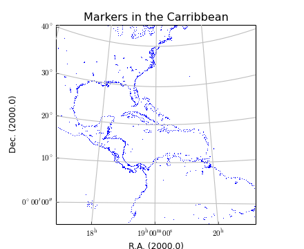
Method maputils.Annotatedimage.positionsfromfile() is based on method tabarray.readColumns(). They share the same parameters which implies that you have many options to get your data from a file.
The next plot also uses tabarray.tabarray to read coast line data. But here we wanted the coast line dots to be connected to get more realistic coast lines. For this we use the comment lines in the file as segment separator. This gives us an option to process the data in segments using tabarray’s segment attribute and avoid that distant segments are connected with straight lines. Again we used the adapted header of the M101 FITS file to scale things up and to set the eye of the ‘hurricane’ in the Caribbean. The example also shows the use of masked arrays for plotting.
Example: mu_hurricane - Hurricane ‘M101’ threatens the Caribbean
1 2 3 4 5 6 7 8 9 10 11 12 13 14 15 16 17 18 19 20 21 22 23 24 25 26 27 28 29 30 31 32 33 34 35 36 37 38 39 40 41 42 43 44 45 46 47 48 49 50 51 52 53 54 55 56 57 58 59 60 61 62 63 | from kapteyn import maputils
from matplotlib import pyplot as plt
from kapteyn import tabarray
import numpy
def plotcoast(fn, pxlim, pylim, col='k'):
coasts = tabarray.tabarray(fn, comchar='s') # Read two columns from file
for segment in coasts.segments:
coastseg = coasts[segment].T
xw = coastseg[1]; yw = coastseg[0] # First one appears to be Latitude
xs = xw; ys = yw # Reset lists which store valid pos.
if 1:
# Mask arrays if outside plot box
xp, yp = annim.projection.topixel((numpy.array(xs),numpy.array(ys)))
xp = numpy.ma.masked_where(numpy.isnan(xp) |
(xp > pxlim[1]) | (xp < pxlim[0]), xp)
yp = numpy.ma.masked_where(numpy.isnan(yp) |
(yp > pylim[1]) | (yp < pylim[0]), yp)
# Mask array could be of type numpy.bool_ instead of numpy.ndarray
if numpy.isscalar(xp.mask):
xp.mask = numpy.array(xp.mask, 'bool')
if numpy.isscalar(yp.mask):
yp.mask = numpy.array(yp.mask, 'bool')
# Count the number of positions in these list that are inside the box
j = 0
for i in range(len(xp)):
if not xp.mask[i] and not yp.mask[i]:
j += 1
if j > 200: # Threshold to prevent too much detail and big pdf's
frame.plot(xp.data, yp.data, color=col)
# Get a header and change some values
f = maputils.FITSimage("m101.fits")
header = f.hdr
header['CDELT1'] = 0.1
header['CDELT2'] = 0.1
header['CRVAL1'] = 285
header['CRVAL2'] = 20
# Use the changed header as external source for new object
f = maputils.FITSimage(externalheader=header, externaldata=f.dat)
fig = plt.figure()
frame = fig.add_subplot(1,1,1)
annim = f.Annotatedimage(frame, cmap="YlGn")
annim.Image()
grat = annim.Graticule()
grat.setp_ticklabel(wcsaxis=0, fmt="%g^{\circ}")
grat.setp_ticklabel(wcsaxis=1, fmt='Dms')
grat.setp_axislabel(plotaxis='bottom', label='West - East')
grat.setp_axislabel(plotaxis='left', label='South - North')
annim.plot()
annim.projection.allow_invalid = True
# Plot coastlines in black, borders in red
plotcoast('WDB/namer-cil.txt', annim.pxlim, annim.pylim, col='k')
plotcoast('WDB/namer-bdy.txt', annim.pxlim, annim.pylim, col='r')
plotcoast('WDB/samer-cil.txt', annim.pxlim, annim.pylim, col='k')
plotcoast('WDB/samer-bdy.txt', annim.pxlim, annim.pylim, col='r')
annim.interact_imagecolors()
plt.show()
|
(Source code, png, hires.png, pdf)
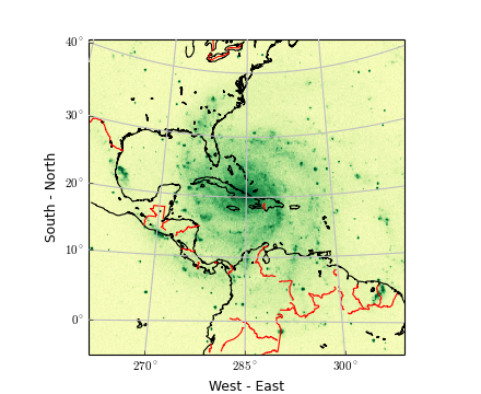
We have two examples of a mosaic of plots. First a mosaic is presented with an image and two position-velocity diagrams. The second is a classic examples which shows channel maps from an HI data cube at different velocities.
The base of the image is a velocity for which we want to show data and a pixel coordinate to set the position of the slice (slicepos=51). This code can be used as a template for a more general application, e.g. with user input of parameters that set velocity and slice position.
Example: mu_channelmaps1.py - Adding two slices
1 2 3 4 5 6 7 8 9 10 11 12 13 14 15 16 17 18 19 20 21 22 23 24 25 26 27 28 29 30 31 32 33 34 35 36 37 38 39 40 41 42 43 44 45 46 47 48 49 50 51 52 53 54 55 56 57 58 59 60 61 62 63 64 65 66 67 68 69 70 71 72 73 74 75 76 77 78 79 80 81 82 | from kapteyn import maputils
from matplotlib import pylab as plt
# This is our function to convert velocity from m/s to km/s
def fx(x):
return x/1000.0
# Create an object from the FITSimage class:
fitsobj = maputils.FITSimage('ngc6946.fits')
# We want to plot the image that corresponds to a certain velocity,
# let's say a radio velocity of 100 km/s
# Find the axis number that corresponds to the spectral axis:
specaxnum = fitsobj.proj.specaxnum
spec = fitsobj.proj.sub(specaxnum).spectra("VRAD-???")
channel = spec.topixel1d(100*1000.0)
channel = round(channel) # We need an integer pixel coordinate
vel = spec.toworld1d(channel) # Velocity near 100 km/s
# Set for this 3d data set the image axes and the position
# for the slice, i.e. the frequency pixel
lonaxnum = fitsobj.proj.lonaxnum
lataxnum = fitsobj.proj.lataxnum
fitsobj.set_imageaxes(lonaxnum,lataxnum, slicepos=channel)
fig = plt.figure(figsize=(7,8))
frame = fig.add_axes([0.3,0.5,0.4,0.4])
annim = fitsobj.Annotatedimage(frame)
annim.Image()
# The FITSimage object contains all the relevant information
# to set the graticule for this image
grat = annim.Graticule()
ruler = annim.Ruler(x1=-51.1916, y1=59.9283, x2=-51.4877, y2=60.2821,
units='arcmin', step=3, mscale=5.0,
color='w', world=True, ha='right')
grat.setp_tick(plotaxis="right", color='r')
pixellabels = annim.Pixellabels(plotaxis=("right","top"), color='r', fontsize=7)
# First position-velocity plot at RA=51
fitsobj.set_imageaxes(lataxnum, specaxnum, slicepos=51)
frame2 = fig.add_axes([0.1,0.3,0.8,0.1])
annim2 = fitsobj.Annotatedimage(frame2)
annim2.set_aspectratio(0.15)
annim2.Image()
grat2 = annim2.Graticule()
grat2.setp_axislabel(plotaxis="right", label='Velocity (km/s)',
fontsize=9, visible=True)
grat2.set_tickmode(plotaxis="right", mode="native_ticks")
grat2.setp_ticklabel(plotaxis="right", fmt="%+5g", fun=fx)
grat2.setp_axislabel("bottom",
label=r"Offset in latitude (arcmin) at $\alpha$ = pixel 51",
fontsize=9)
grat2.setp_axislabel(plotaxis="left", visible=False)
grat2.set_tickmode(plotaxis="left", mode="no_ticks")
annim2.Pixellabels(plotaxis=("top", "left"))
# Second position-velocity plot at DEC=51
fitsobj.set_imageaxes(lonaxnum, specaxnum, slicepos=51)
frame3 = fig.add_axes([0.1,0.1,0.8,0.1])
annim3 = fitsobj.Annotatedimage(frame3)
annim3.set_aspectratio(0.15)
annim3.Image()
grat3 = annim3.Graticule()
grat3.setp_axislabel("right",
label='Velocity (km/s)', fontsize=9, visible=True)
grat3.set_tickmode(plotaxis='right', mode="native_ticks")
# The next line forces labels to be right aligned, but one needs a shift
# in x to set the labels outside the plot
grat3.setp_ticklabel(plotaxis="right", fmt="%8g", fun=fx, ha="right", x=1.075)
grat3.setp_axislabel(plotaxis="left", visible=False)
grat3.set_tickmode(plotaxis="left", mode="no_ticks")
grat3.setp_axislabel("bottom",
label=r"Offset in longitude (arcmin) at $\delta$ = pixel 51",
fontsize=9)
annim3.Pixellabels(plotaxis=("top", "left"))
# Set title and adjust position of title
frame.set_title('NGC 6946 at %g km/s (channel %d)' % (vel/1000.0, channel), y=1.1)
maputils.showall()
|
(Source code, png, hires.png, pdf)
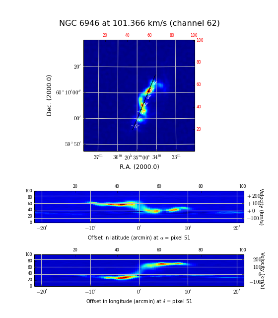
For a series of so called channel maps we use Matplotlib’s add_subplot() to position the plots automatically. To set the same scale for the colors in each plot, we first calculate the minimum and maximum values in the data with maputils.FITSimage.get_dataminmax(). The scale itself is set with parameters clipmin and clipmax in the constructor of maputils.Annotatedimage.
Before you make a hardcopy, it is possible to fine tune the colors because for each plot both mouse and key interaction is added with maputils.Annotatedimage.interact_imagecolors(). Some channels seem not to contain any signal but when you fine tune the colors you discover that they show features. For inspection one can set histogram equalization on/off for each plot separately. Special attention is paid to put labels in the plots with velocity information.
Also this example turns out to be a small but practical tool to inspect data.
Example: mu_channelmosaic.py - A mosaic of channelmaps
1 2 3 4 5 6 7 8 9 10 11 12 13 14 15 16 17 18 19 20 21 22 23 24 25 26 27 28 29 30 31 32 33 34 35 36 37 38 39 40 41 42 43 44 45 46 47 48 49 50 | from kapteyn import maputils
from matplotlib import pylab as plt
# This is our function to convert velocity from m/s to km/s
def fx(x):
return x/1000.0
# Create an object from the FITSimage class:
fitsobj = maputils.FITSimage('ngc6946.fits')
specaxnum = fitsobj.proj.specaxnum
lonaxnum = fitsobj.proj.lonaxnum
lataxnum = fitsobj.proj.lataxnum
spec = fitsobj.proj.sub(specaxnum).spectra("VRAD-???")
start = 5; end = fitsobj.proj.naxis[specaxnum-1]; step = 4
channels = range(start,end,step)
nchannels = len(channels)
fig = plt.figure(figsize=(7,8))
fig.subplots_adjust(left=0, bottom=0, right=1, top=1, wspace=0, hspace=0)
vmin, vmax = fitsobj.get_dataminmax()
print "Vmin, Vmax of data in cube:", vmin, vmax
cmap = 'spectral' # Colormap
cols = 5
rows = nchannels / cols
if rows*cols < nchannels: rows += 1
for i, ch in enumerate(channels):
fitsobj.set_imageaxes(lonaxnum, lataxnum, slicepos=ch)
print "Min, max in this channel: ", fitsobj.get_dataminmax(box=True)
frame = fig.add_subplot(rows, cols, i+1)
mplim = fitsobj.Annotatedimage(frame,
clipmin=vmin, clipmax=vmax,
cmap=cmap)
mplim.Image()
vel = spec.toworld1d(ch)
velinfo = "ch%d = %.1f km/s" % (ch, vel/1000.0)
frame.text(0.98, 0.98, velinfo,
horizontalalignment='right',
verticalalignment='top',
transform = frame.transAxes,
fontsize=8, color='w',
bbox=dict(facecolor='red', alpha=0.5))
mplim.plot()
if i == 0:
cmap = mplim.cmap
mplim.interact_imagecolors()
plt.show()
|
(Source code, png, hires.png, pdf)
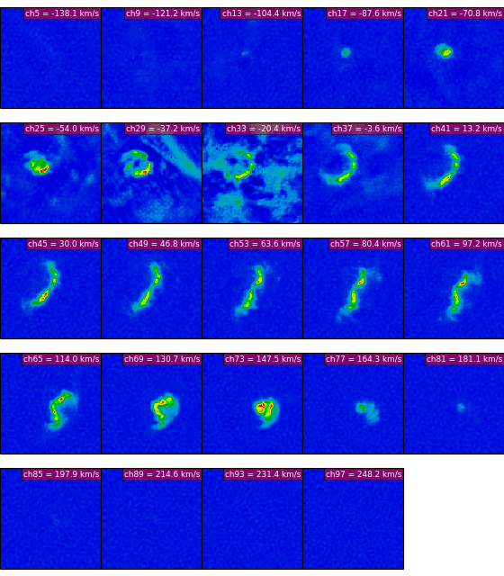
Matplotlib (v 0.99) provides a number of built-in keyboard shortcuts. These are available on any Matplotlib window. Most of these shortcuts start actions that can also be started with buttons on the canvas. Also some keys interfere with the system and others don’t seem to work for certain combinations of Matplotlib version and backend. Therefore a filter is applied to those shortcuts and now you need to specify the keys from the table below for which you want to use the shortcut with a function:
>>> from kapteyn.mplutil import KeyPressFilter
>>> KeyPressFilter.allowed = ['f', 'g', 'l']
Note that the interactions defined in module maputils could interfere with some of these keys. By default, the keys ‘f’ and ‘g’ are allowed.
Some Matplotlib Navigation Keyboard Shortcuts
| Command | Keyboard Shortcut(s) |
|---|---|
| Toggle fullscreen | f |
| Toggle grid | g |
| Toggle y axis scale (log/linear) | l |
Three methods from maputils.Annotatedimage add mouse and keyboard interaction. These methods are described in the next sections:
Method maputils.Annotatedimage.interact_imagecolors() adds keys and mouse interaction for color editing i.e. change color scheme and settings for image and colorbar. The active keys are:
| Command | Keyboard Shortcut(s) |
|---|---|
| Colormap scaling linear | 1 |
| Colormap scaling logarithmic | 2 |
| Colormap scaling exponential | 3 |
| Colormap scaling square root | 4 |
| Colormap scaling square | 5 |
| Toggle between data and histogram equalized version | h |
| Loop forward through list with colormaps | page-up |
| Loop backwards through list with colormaps | page-down |
| Save current colormap to disk | m |
| Toggle between inverse and normal scaling | 9 (nine) |
| reset the colors to start values | 0 (zero) |
| Change color of bad pixels (blanks) | b |
The right mouse button must be pressed to change slope and offset of the function that maps image values to colors in the current color map.
Example: mu_smooth.py - Apply Gaussian filter
Smoothing of images is a technique that is often used to enhance the contrast of extended emission. Maputils provides a method for smoothing using a gaussian kernel. The method expects values for the dispersion of the Gauss in both directions x and y. To show how this can be used interactively, we give a small script where a Matplotlib Slider object changes the value of sigma (which is copied for both the x and y direction).
1 2 3 4 5 6 7 8 9 10 11 12 13 14 15 16 17 18 19 20 21 22 23 24 25 26 | from kapteyn import maputils
from matplotlib import pyplot as plt
from matplotlib.widgets import Slider
def func(x):
nx = ny = x
annim.set_blur(True, nx, ny, new=True)
f = maputils.FITSimage("m101.fits")
fig = plt.figure(figsize=(9,7))
frame = fig.add_subplot(1,1,1)
fr2 = fig.add_axes([0.3,0.01,0.4,0.03])
valinit = 1.0
sl = Slider(fr2, "Sigma: ", 0.1, 5.0, valinit=valinit)
sl.on_changed(func)
annim = f.Annotatedimage(frame)
#annim.set_colormap("mousse.lut")
annim.Image()
annim.plot()
func(valinit)
annim.interact_toolbarinfo()
annim.interact_imagecolors()
annim.interact_writepos()
plt.show()
|
(Source code, png, hires.png, pdf)

Method maputils.Annotatedimage.interact_toolbarinfo() connects movements of your mouse to messages in the toolbar of your canvas. The message shows pixel position, the corresponding world coordinates, and the image value of the pixel.
Note
There is a minimum width for the window to be able to display the message. If you see any imcomplete text, then resize the window until it is wide enough to show the message.
A programmer can change the formatting of the informative string using parameters with the same name as the attributes of an object from class maputils.Annotatedimage.Positionmessage If a format is set to None, its corresponding number(s) will not appear in the informative message. Here is an example how to skip the world coordinates (wcsfmt=None) and to add a format for the image values (zfmt).
>>> interact_toolbarinfo(wcsfmt=None, zfmt="%g")
Method maputils.Annotatedimage.interact_writepos() writes the toolbar message with information about coordinates and image values to the terminal. This is a primitive way to collect positional information about features in a map.
>>> x,y= 196.4, 303.5  wcs=210.858423, 54.365281  Z=+8.74e+03
>>> x,y= 260.5, 378.3  wcs=210.806913, 54.400918  Z=+4.75e+03
>>> x,y= 391.1, 231.1  wcs=210.700135, 54.331856  Z=+6.08e+03
The first two numbers are the x and y pixel coordinate. Then two numbers follow which represent the pixel position in world coordinates. The units are the S.I. versions of the units found in the header. For spatial maps these units are degrees. The values are the real longitude and latitude even when the labels along the axes represent offsets. For spectral axes, the units depend on the selected spectral translation.
Here is a minimalistic example how to add user interaction:
1 2 3 4 5 6 7 8 9 10 11 12 13 14 15 16 17 18 19 20 21 22 23 24 25 26 27 28 29 30 | """Show interaction options"""
from kapteyn import maputils
from matplotlib import pyplot as plt
from kapteyn.mplutil import KeyPressFilter
KeyPressFilter.allowed = ['f','g', 'l']
f = maputils.FITSimage("m101.fits")
#f.set_limits((100,500),(200,400))
fig = plt.figure(figsize=(9, 7))
frame = fig.add_subplot(1, 1, 1)
mycmlist = ["mousse.lut", "ronekers.lut"]
maputils.cmlist.add(mycmlist)
print "Colormaps: ", maputils.cmlist.colormaps
mplim = f.Annotatedimage(frame, cmap="mousse.lut")
mplim.cmap.set_bad('w')
ima = mplim.Image()
mplim.Pixellabels()
mplim.Colorbar()
mplim.plot()
mplim.interact_toolbarinfo()
mplim.interact_imagecolors()
mplim.interact_writepos()
plt.show()
|
For a formatted output one could add parameters to interact_writepos(). The next line writes no pixel coordinates, writes spatial coordinates in degrees (not in HMS/DMS format) and adds a format for the world coordinates and the image value(s).
>>> interact_writepos(pixfmt=None, wcsfmt="%.12f", zfmt="%.3e", hmsdms=False)
Or if you need a lot of precision in the seconds of a HMS/DMS format:
>>> interact_writepos(dmsprec=3)
Another powerful tool of the maputils module is (together with module shapes) the option to propagate geometric shapes plotted in one image to other images from a list with images. A user selects a shape from the list Polygon, Ellipse, Circle, Rectangle and Spline, and interactively changes the geometry of a shape in an arbitray image in a mosaic of images. Then this shape duplicates itself in pixel coordinates or world coordinates on the other images. If we use the default setting then the duplication is in world coordinates, meaning that for different projections the geometry is different, but both represent the same area in the sky.
Note
If we change the image for interaction with circles or ellipses then their shape will change to the best approach of a circle or an ellipse for the new image and the deviation in geometry appears in the other image(s). This does not apply to the situation where we duplicate shapes in pixel coordinates.
For these areas the flux can be calculated. By default the flux is given by the (lambda) expression s/a where s represents the sum of the intensities of all the pixels enclosed by area a. One can supply a user defined function or lambda expression using Annotatedimage attribute fluxfie. Sometimes more precision is required. Then one can subdivide pixels using Annotatedimage attribute pixelstep.
1 2 3 4 5 6 7 8 9 10 11 12 13 14 15 16 17 18 19 20 21 22 23 24 25 26 27 28 29 30 31 32 33 34 35 36 37 38 39 40 41 42 43 44 45 46 47 48 49 50 | from kapteyn import maputils, shapes
from matplotlib import pyplot as plt
Basefits = maputils.FITSimage("m101big.fits")
hdr = Basefits.hdr.copy()
hdr['CTYPE1'] = 'RA---MER'
hdr['CTYPE2'] = 'DEC--MER'
hdr['CRVAL1'] = 0.0
hdr['CRVAL2'] = 0.0
naxis1 = Basefits.hdr['NAXIS1']
naxis2 = Basefits.hdr['NAXIS2']
# Get an estimate of the new corners
x = [0]*5; y = [0]*5
x[0], y[0] = Basefits.proj.toworld((1,1))
x[1], y[1] = Basefits.proj.toworld((naxis1,1))
x[2], y[2] = Basefits.proj.toworld((naxis1,naxis2))
x[3], y[3] = Basefits.proj.toworld((1,naxis2))
x[4], y[4] = Basefits.proj.toworld((naxis1/2.0,naxis2))
# Create a dummy object to calculate pixel coordinates
# in the new system. Then we can find the area in pixels
# that corresponds to the area in the sky.
f = maputils.FITSimage(externalheader=hdr)
px, py = f.proj.topixel((x,y))
pxlim = [int(min(px))-10, int(max(px))+10]
pylim = [int(min(py))-10, int(max(py))+10]
Reprojfits = Basefits.reproject_to(hdr, pxlim_dst=pxlim, pylim_dst=pylim)
fig = plt.figure(figsize=(14,9))
frame1 = fig.add_axes([0.07,0.1,0.35, 0.8])
frame2 = fig.add_axes([0.5,0.1,0.43, 0.8])
im1 = Basefits.Annotatedimage(frame1)
im1.set_blankcolor('k')
im2 = Reprojfits.Annotatedimage(frame2)
im1.Image(); im1.Graticule()
im2.Image(); im2.Graticule()
im1.plot(); im2.plot()
im1.interact_imagecolors(); im1.interact_toolbarinfo()
im2.interact_imagecolors(); im2.interact_toolbarinfo()
#im1.fluxfie = lambda s, a: s/a
#im2.fluxfie = lambda s, a: s/a
im1.pixelstep = 0.2
im2.pixelstep = 0.5
images = [im1, im2]
shapes = shapes.Shapecollection(images, fig, wcs=True, inputwcs=True)
plt.show()
|
Your Matplotlib figure with one or more images gets a number of buttons at the top of your figure. You should anticipate on this when setting the figure size. Ofcourse one can also resize the plot window to make space for the buttons. The gui is simple. Here is an example. It corresponds to the example script above. A re-projection (to Mercator) of M101 (with exaggerated values for the pixel sizes) is displayed together with the original image. One ellipse is plotted to demonstrate that the same area in the re-projection looks different. If enough resolution (pixelstep=0.2) is used, then the flux in both shapes is comparable.
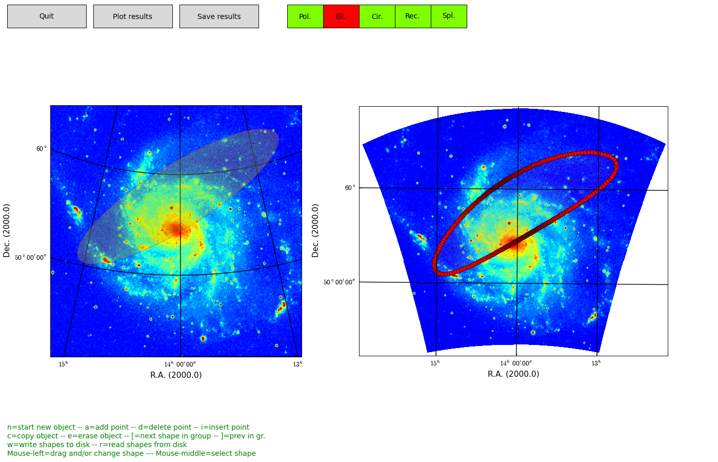
Fig. – Calculate flux in user defined shapes in images with different world coordinate systems.
In the constructor of maputils.Annotatedimage one can set a color map with keyword cmap. There are four options here:
| Option | Example |
|---|---|
| Matplotlib color map (string) | cmap=’jet’ |
| Path and filename of color map on disk | cmap=’/home/user/myluts/rainbow4.lut’ |
| A Color map from the Kapteyn Package | cmap=’ronekers.lut’ |
| Instance of class mplutil.VariableColormap | cmap=myimage.cmap |
Module maputils has a global list called cmlist which contains the colormaps provided by Matplotlib. You can add an external colormap to this list as follows:
>>> maputils.cmlist.add('/home/user/luts/rainbow4.lut')
It will be prepended to the existing list. One can also prepend multiple external colormaps assembled in a list. This list can also be compiled from the color maps available in the Kapteyn Package. If you have a number of local color maps then use Python’s glob function to read them all (or a selection) as in the next example:
1 2 3 4 5 6 7 8 9 10 11 12 13 14 15 16 17 18 19 20 21 22 23 24 25 26 27 28 29 30 31 32 33 34 35 36 37 38 39 40 | from kapteyn import maputils
from matplotlib import pyplot as plt
from kapteyn import mplutil
import glob
f = maputils.FITSimage("m101.fits")
fig = plt.figure(figsize=(9,7))
frame = fig.add_axes([0.1,0.2,0.85, 0.75])
extralist = mplutil.VariableColormap.luts()
print "Extra luts from Kapteyn Package", extralist
maputils.cmlist.add(extralist)
mycmlist = glob.glob("*.lut")
print "\nFound private color maps:", mycmlist
maputils.cmlist.add(mycmlist)
print "\nAll color maps now available: ", maputils.cmlist.colormaps
annim = f.Annotatedimage(frame) #,cmap="mousse.lut")
annim.set_colormap("mousse.lut")
annim.Image()
annim.Pixellabels()
annim.Colorbar()
annim.plot()
annim.interact_toolbarinfo()
annim.interact_imagecolors()
annim.interact_writepos()
units = 'unknown'
if 'BUNIT' in f.hdr:
units = f.hdr['BUNIT']
helptext = "File: [%s] Data units: [%s]\n" % (f.filename, units)
helptext += annim.get_colornavigation_info()
tdict = dict(color='g', fontsize=10, va='bottom', ha='left')
fig.text(0.01,0.01, helptext, tdict)
plt.show()
|
(Source code, png, hires.png, pdf)

The format of a colormap on disk (also called a color LookUp Table or lut) is simple. There should be a number (e.g. 256) lines with three floating point numbers between 0 and 1 which represent Red, Green and Blue.
1 2 3 4 5 6 7 8 9 10 11 12 13 14 15 16 17 18 19 20 21 22 23 24 25 26 27 28 29 30 31 32 33 34 35 36 | from kapteyn import maputils
from matplotlib import pyplot as plt
from numpy import mgrid,exp
f = maputils.FITSimage("m101.fits")
n1, n2 = f.proj.naxis
X,Y = mgrid[0:n1, 0:n2]
Z = exp( -(X**2)/1.0e5-(Y**2)/1.0e5 )
f2 = maputils.FITSimage(externalheader=f.hdr, externaldata=Z)
fig = plt.figure()
frame = fig.add_subplot(1,2,1)
annim = f2.Annotatedimage(frame)
annim.set_colormap("rainbow.lut")
annim.cmap.set_length(64)
annim.Image()
annim.Pixellabels()
annim.Colorbar(fontsize=7, orientation='horizontal')
annim.plot()
annim.interact_toolbarinfo()
annim.interact_imagecolors()
annim.interact_writepos()
frame2 = fig.add_subplot(1,2,2)
annim2 = f2.Annotatedimage(frame2)
annim2.set_colormap("rainbow.lut")
annim2.cmap.set_length(1021)
annim2.Image()
annim2.Pixellabels()
annim2.Colorbar(fontsize=7, orientation='horizontal')
annim2.plot()
annim2.interact_toolbarinfo()
annim2.interact_imagecolors()
annim2.interact_writepos()
plt.show()
|
(Source code, png, hires.png, pdf)
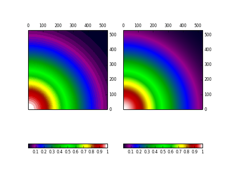
In this plot we demonstrate the difference between a small color map (64 color entries) and a big color map (1021 entries). The plot on the left uses the small color map. What you should observe are the false contours because that color map does not have the enough resolution to show smooth transitions between colors. The plot on the right has a big color map and there you don’t see these transitions.
Note
The default length of a color map is 256. With this length the effect of steps in the color gradient is less obvious but still there. You should only extend your color map if a high resolution is required.
If you modify the default colors in an image and want to be able to restore the exact color scheme in a second run, then save the modified colormap to disk with key ‘m’. Note that we assume you connected mouse and keyboard interaction with maputils.Annotatedimage.interact_imagecolors(). The file on disk will get the name of the FITS file that you opened (or an alternative if you used external header and image data) followed by the extension .lut. This colormap can be used as external colormap to restore the adjusted colors.
There are at least two circumstances where one wants to share a colormap between multiple images. The first is the movie loop of images and the second is when we have a mosaic of channel maps. A change in the colormap settings affects all images in the movie or in the mosaic. There could be exceptions where you want each image to have its own colormap, but usually it is more convenient to share it. The trick is to use a loop over all images and to set the colormap for the first image and copy this colormap for the others. Have a look at the examples that illustrate movies and mosaics:
1 2 3 4 5 6 7 8 9 10 11 | cmap = 'spectral'
for i, ch in enumerate(channels):
fitsobj.set_imageaxes(lonaxnum, lataxnum, slicepos=ch)
frame = fig.add_subplot(rows, cols, i+1)
mplim = fitsobj.Annotatedimage(frame, clipmin=vmin, clipmax=vmax,
cmap=cmap)
mplim.Image()
mplim.plot()
if i == 0:
cmap = mplim.cmap # Copy map to set for other images
mplim.interact_imagecolors()
|
An image can contain some ‘bad pixels’. A bad pixel is a location where a physical value is missing. These pixels are represented by the value NaN. For FITS files where the data are integers (i.e. keyword BITPIX has a positive value) one needs to set an integer value for a bad pixel with FITS keyword BLANK. For the extraction of data the package PyFITS is used. PyFITS should take care of blanks automatically.
Some FITS writers use for BITPIX=-32 a blank value equal to -inf. To avoid problems with plotting images and contours we replace these values in the data with NaN’s first before anything is plotted.
In the next example we inserted some blank values. They appear as a square in the middle of the image. The color of a blank pixel is either set in the constructor of maputils.Annotatedimage with keyword blankcolor, or it can be changed with key ‘b’ if we applied user interaction with maputils.Annotatedimage.interact_imagecolors().
1 2 3 4 5 6 7 8 9 10 11 12 13 14 15 16 17 18 19 20 21 22 23 24 25 26 27 28 29 | from kapteyn import maputils
from matplotlib import pyplot as plt
from matplotlib.colors import LogNorm
import glob
f = maputils.FITSimage("blanksetmin32.fits")
#f = maputils.FITSimage("blankset16.fits")
f.set_imageaxes(1,2)
fig = plt.figure(figsize=(9,7))
frame = fig.add_subplot(1,1,1)
mycmlist = ["mousse.lut", "ronekers.lut"]
maputils.cmlist.add(mycmlist)
print "Colormaps: ", maputils.cmlist.colormaps
mplim = f.Annotatedimage(frame, cmap="mousse.lut", blankcolor='w')
mplim.Image()
#mplim.Image()
#mplim.set_blankcolor('c')
mplim.Pixellabels()
mplim.Colorbar()
mplim.plot()
mplim.interact_toolbarinfo()
mplim.interact_imagecolors()
mplim.interact_writepos()
plt.show()
|
If you change the input FITS file from blanksetmin32.fits to blankset16.fits, then you get the same image and the same blanks, which proves that the blanks can also be read from a FITS file with scaled data.
In version 2.3 of the Kapteyn Package, a lot of effort was spent on developing a class for access to- and visualization of N dimensional data. This visualization is restricted to a movieloop of images and side panels with slices from a data cube. One can change the color mapping interactively and graticules can be overlayed.
The base class for interactive image viewing is maputils.Cubes. It needs only a Figure instance for its initialization. There are a couple of extra parameters. One is helptext which shows a informative text on your plot to help you with the interaction. The other is imageinfo which must be set to True if you want a line in your plot with text showing which slice is on display by giving the name and world coordinate of the repeat axes.
The core of interactive image display is maputils.Cubes. An object of this class is constructed with:
>>>   myCubes = Cubes(fig, toolbarinfo=True, printload=False,
>>>                        helptext=False, imageinfo=True)
1 2 3 4 5 6 7 8 9 10 11 12 13 14 15 16 17 18 19 20 | #!/usr/bin/env python
from kapteyn import wcsgrat, maputils
from matplotlib.pyplot import figure, show
fig = figure()
myCubes = maputils.Cubes(fig, toolbarinfo=True, printload=False,
helptext=False, imageinfo=True)
# Create a maputils FITS object from a FITS file on disk
fitsobject = maputils.FITSimage('ngc6946.fits')
naxis3 = fitsobject.hdr['NAXIS3']
# Note that slice positions follow FITS syntax, i.e. start at 1
slicepos = range(1,naxis3+1)
frame = fig.add_subplot(1,1,1)
vmin, vmax = fitsobject.get_dataminmax()
cube = myCubes.append(frame, fitsobject, (1,2), slicepos,
vmin=vmin, vmax=vmax, hasgraticule=True)
show()
|
An object from class maputils.Annotatedimage has a so called wcs projection object (see module wcs) as attribute (called projection) This projection object has methods for the transformation between pixel- and world coordinates. In the context of module maputils there are two convenience methods with the same name and same functionality i.e. maputils.Annotatedimage.toworld() and maputils.Annotatedimage.topixel(). But in maputils we deal with two dimensional structures only, so these methods are easier to use. Look at the next example to find out how you can use them
1 2 3 4 5 6 7 8 9 10 11 12 13 | from kapteyn import maputils
# The set is 3-dim. but default the first two axes are
# used to extract the image data
f = maputils.FITSimage("ngc6946.fits")
annim = f.Annotatedimage()
x = 200; y = 350
lon, lat = annim.toworld(x,y)
print "lon, lat =", lon, lat
x, y = annim.topixel(lon, lat)
print "x, y = ", x, y
|
Module maputils supports the extraction of data slices in any direction. This enables you to inspect maps with for example one spatial axis and one spectral axis (so called position velocity map). For conversions between pixel- and world coordinates we need a matching spatial axis to process the transformation. The methods used in the previous example can be used to get values for the matching axis also. One only needs to set parameter matchspatial to True:
1 2 3 4 5 6 7 8 9 10 11 12 13 14 15 16 17 18 19 | from kapteyn import maputils
f = maputils.FITSimage("ngc6946.fits")
# Get an XV slice at DEC=51
f.set_imageaxes(1,3, slicepos=51)
annim = f.Annotatedimage()
# Which pixel coordinates correspond to CRVAL's?
crpix = annim.projection.crpix
print "CRPIX from header", crpix
# Convert these to world coordinates
x = crpix[0]; y = crpix[1]
lon, velo, lat = annim.toworld(x, y, matchspatial=True)
print "lon, velo, lat =", lon, velo, lat
print "Should be equivalent to CRVAL:", annim.projection.crval
x, y, slicepos = annim.topixel(lon, velo, matchspatial=True)
print "Back to pixel coordinates: x, y =", x, y, slicepos
|
Note that we can modify the FITS object ‘f’ in the example so that instead of velocities we get corresponding frequencies. Add a spectral translation with method maputils.FITSimage.set_spectrans() as in:
>>> f = maputils.FITSimage("ngc6946.fits")
>>> f.set_imageaxes(1,3, slicepos=51)
>>> f.set_spectrans("FREQ-???")
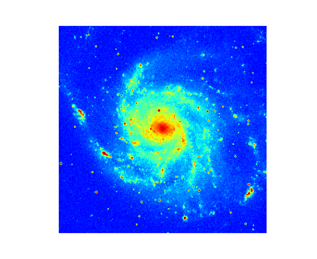
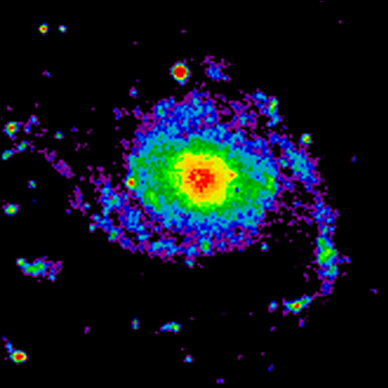
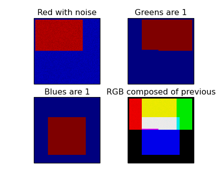
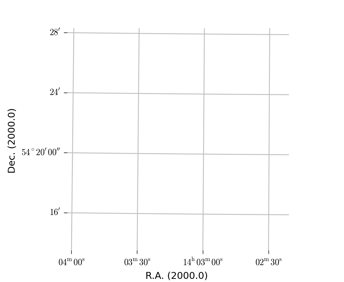
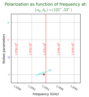
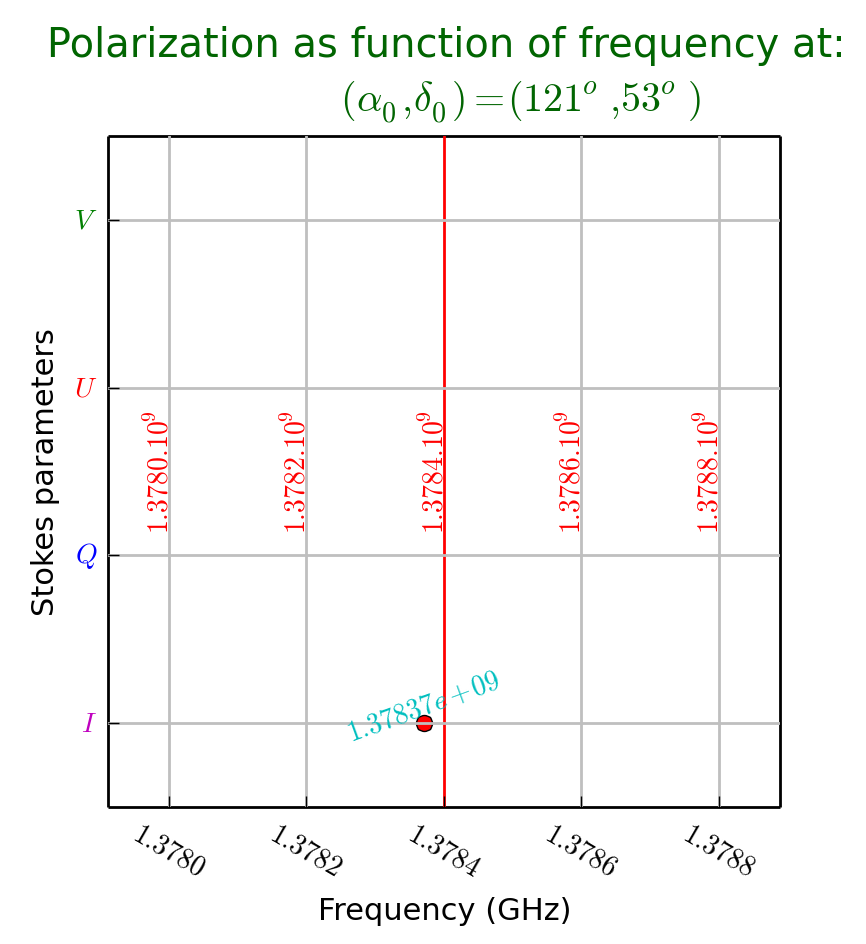
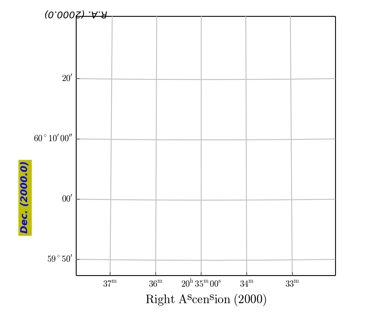
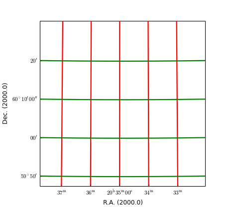
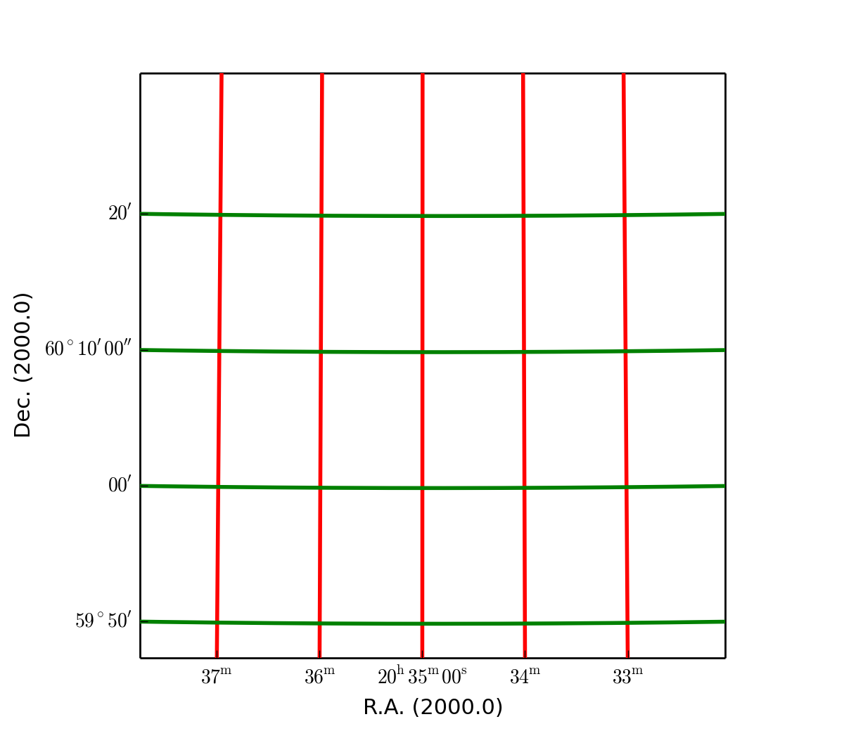
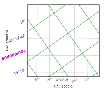
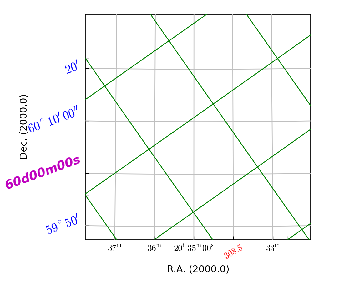
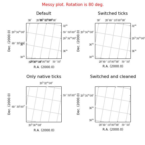
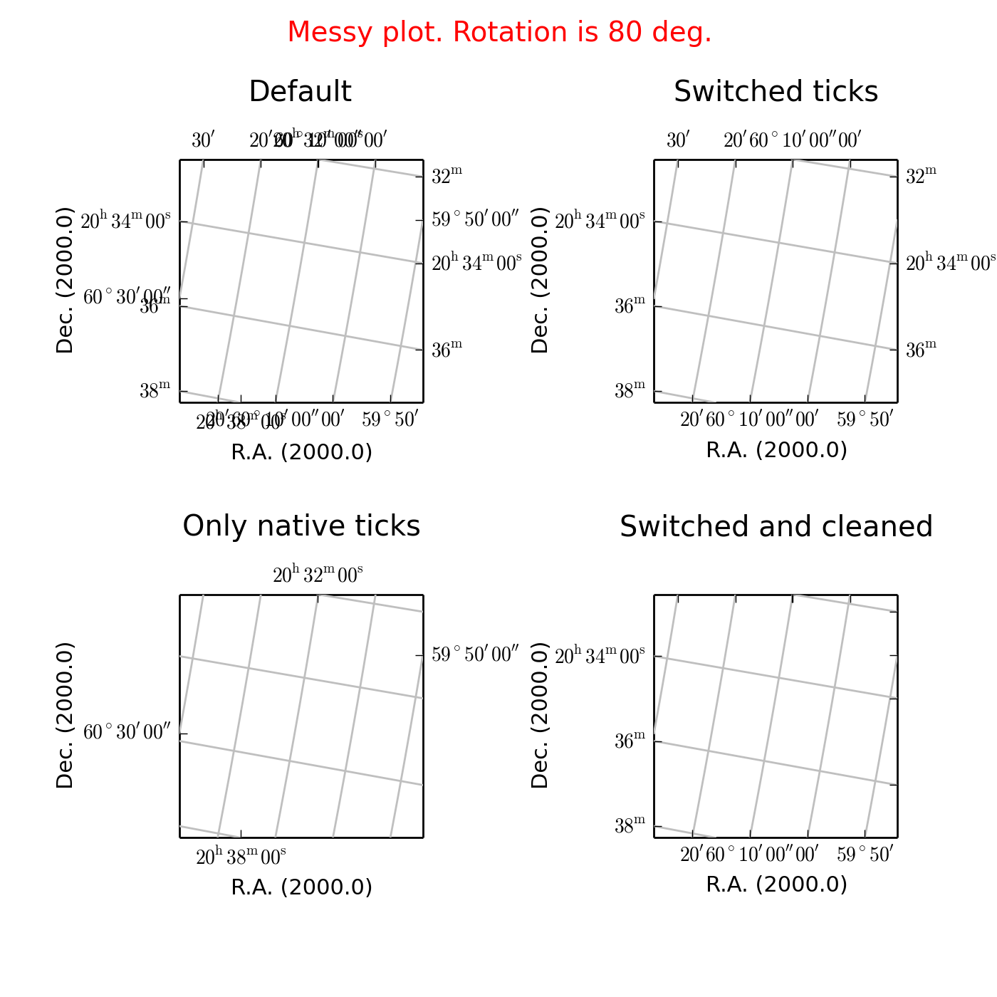
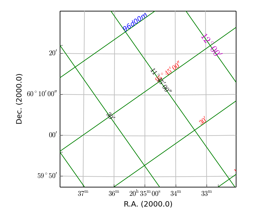
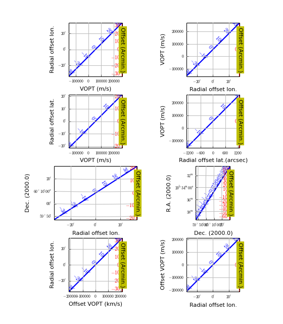
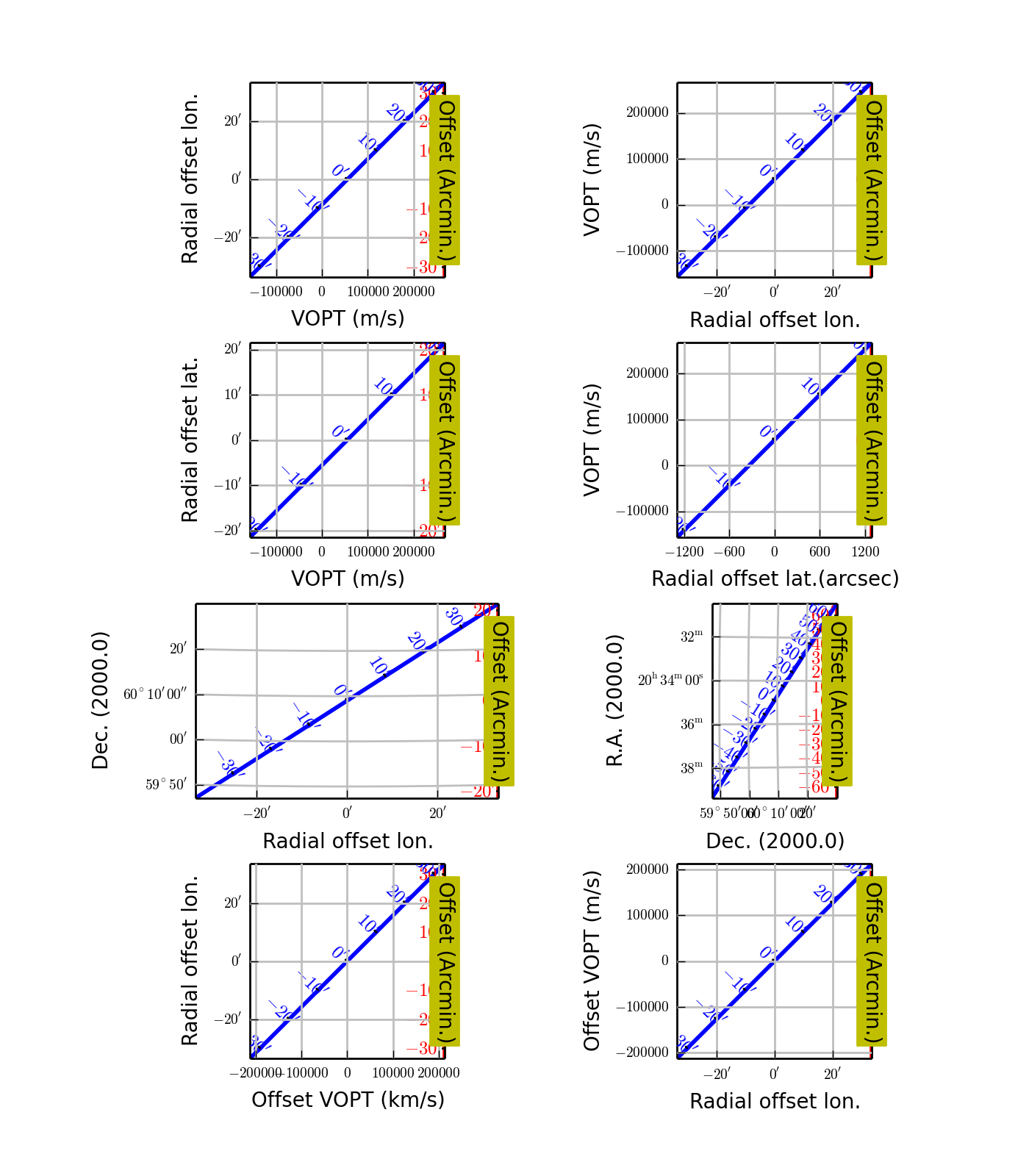
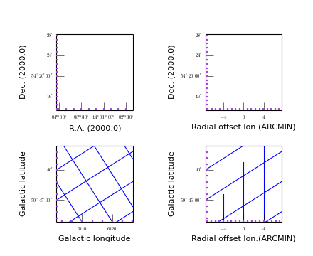
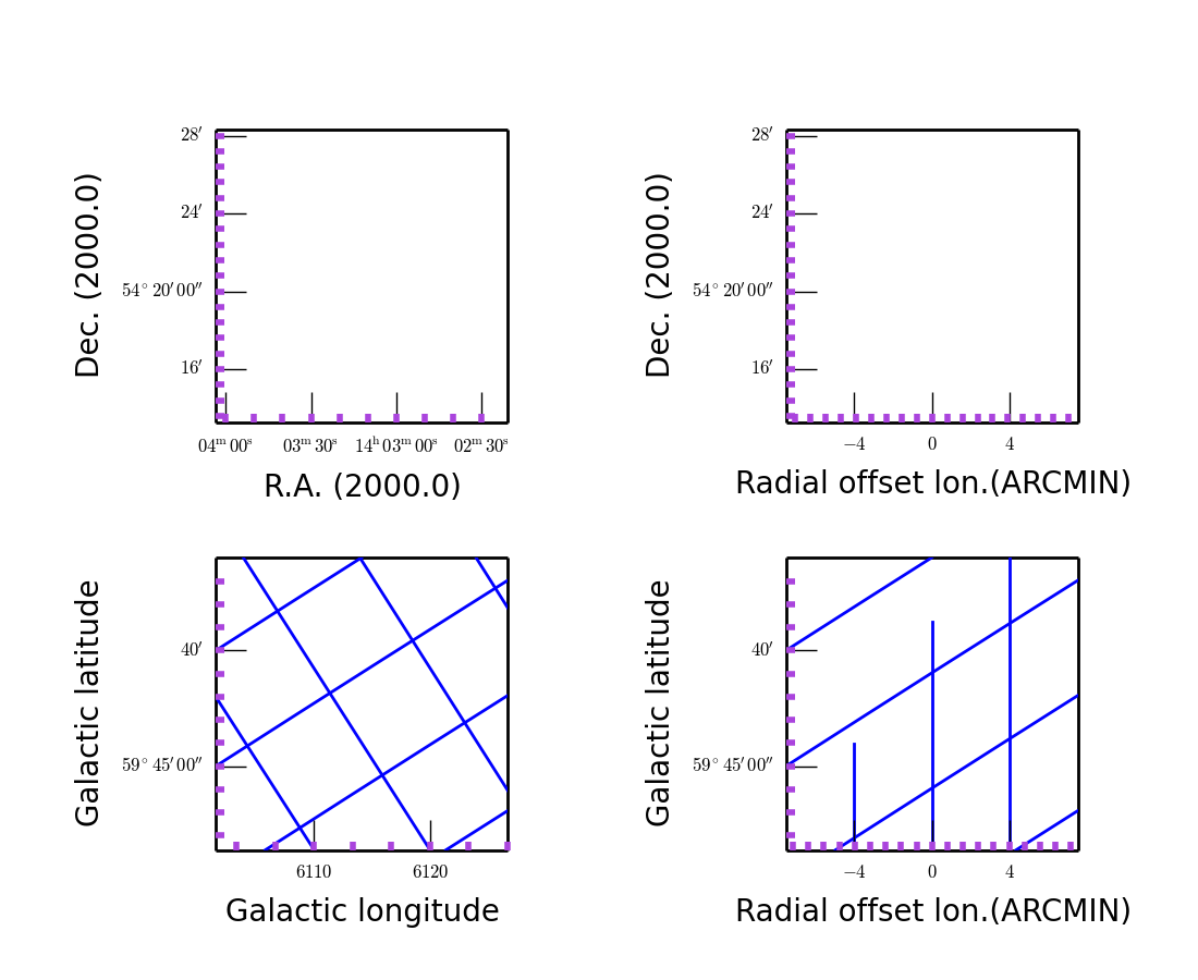
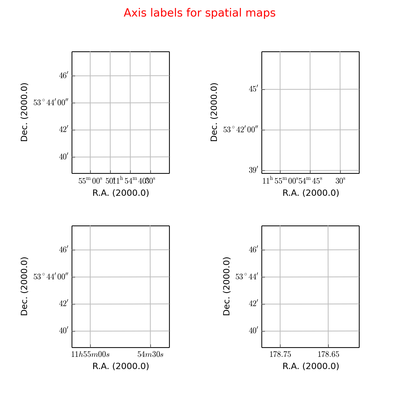
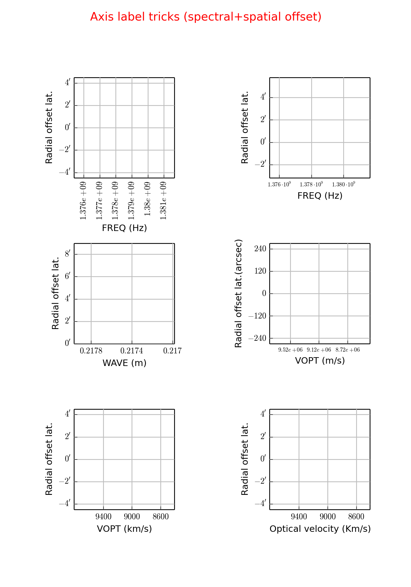
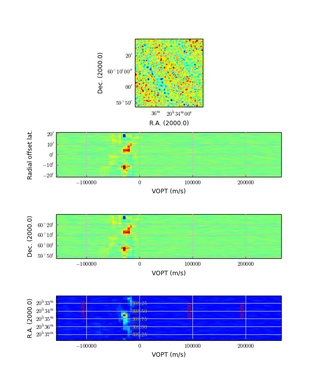
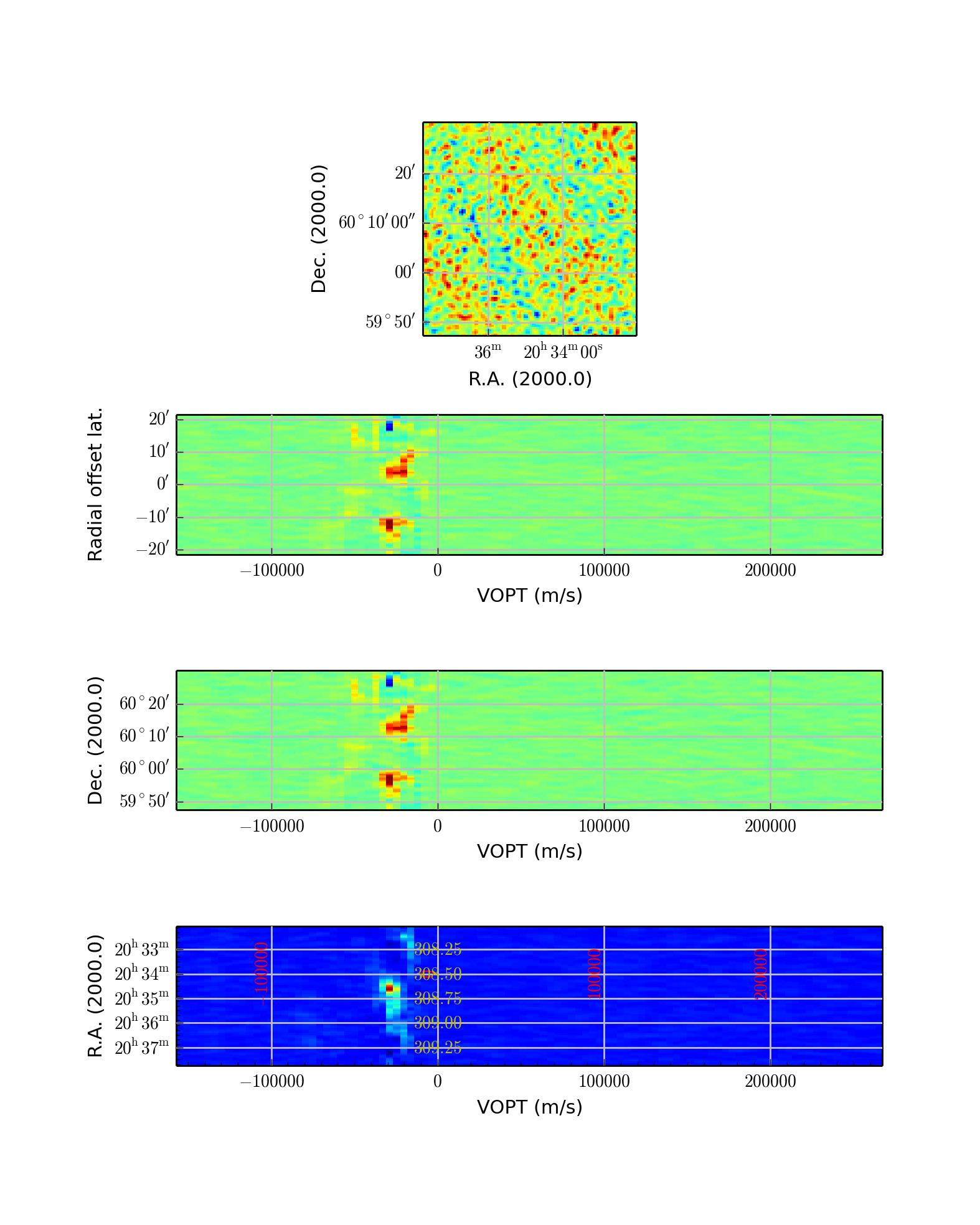
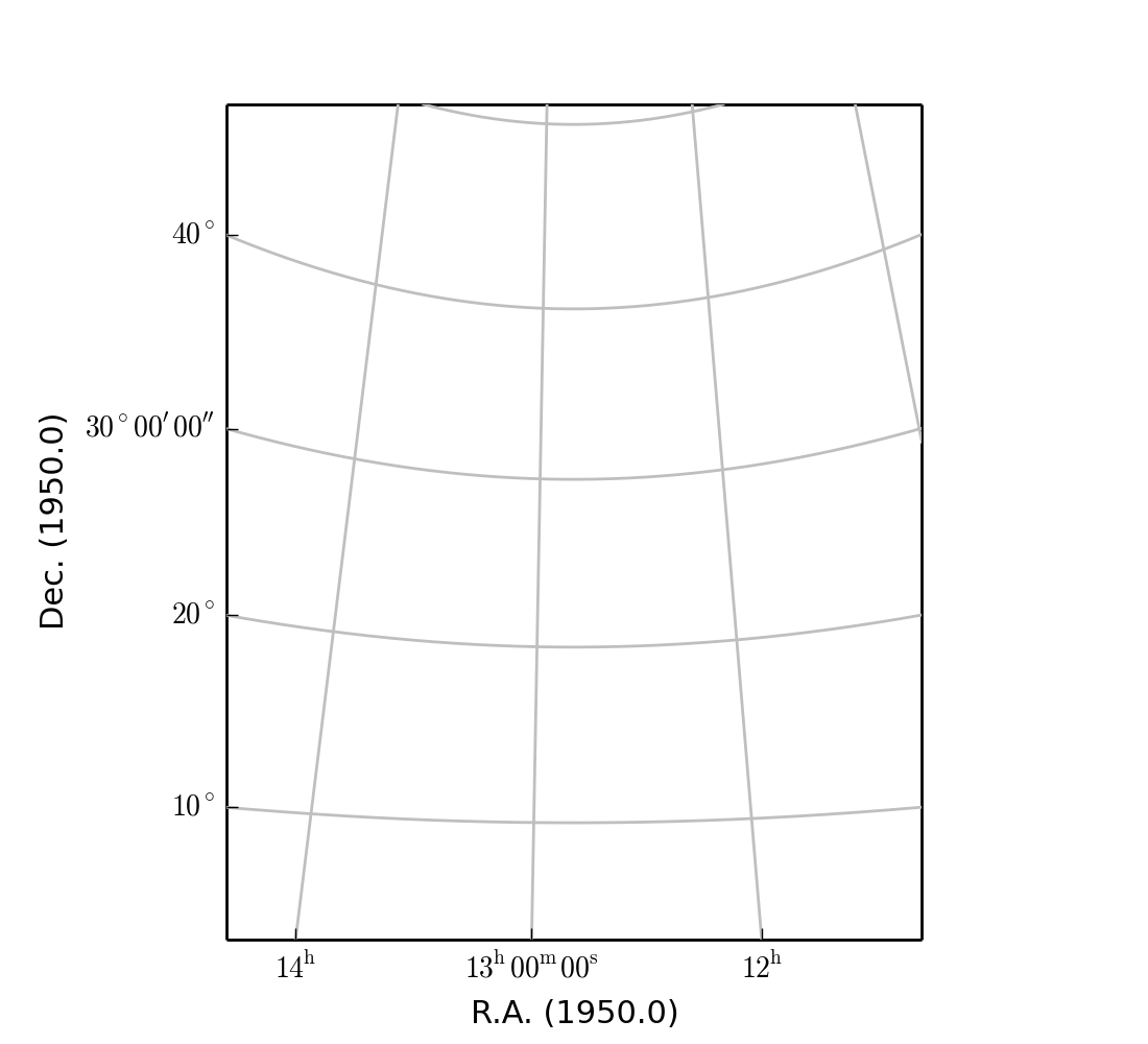
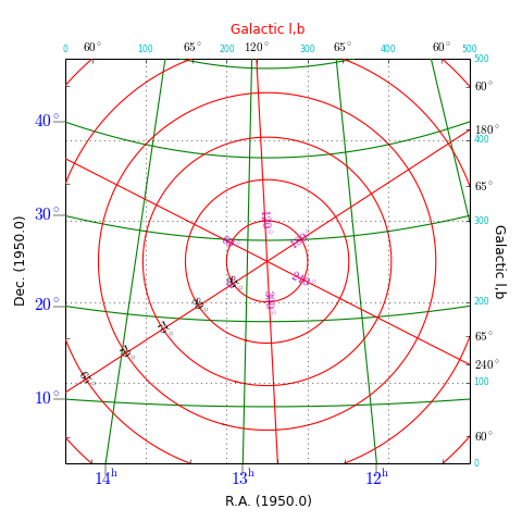
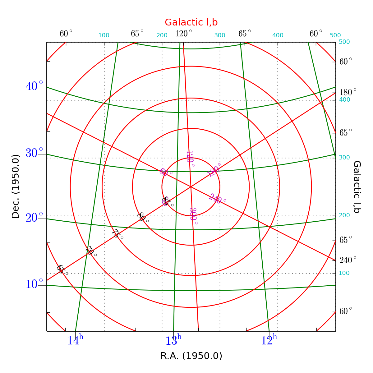
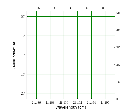
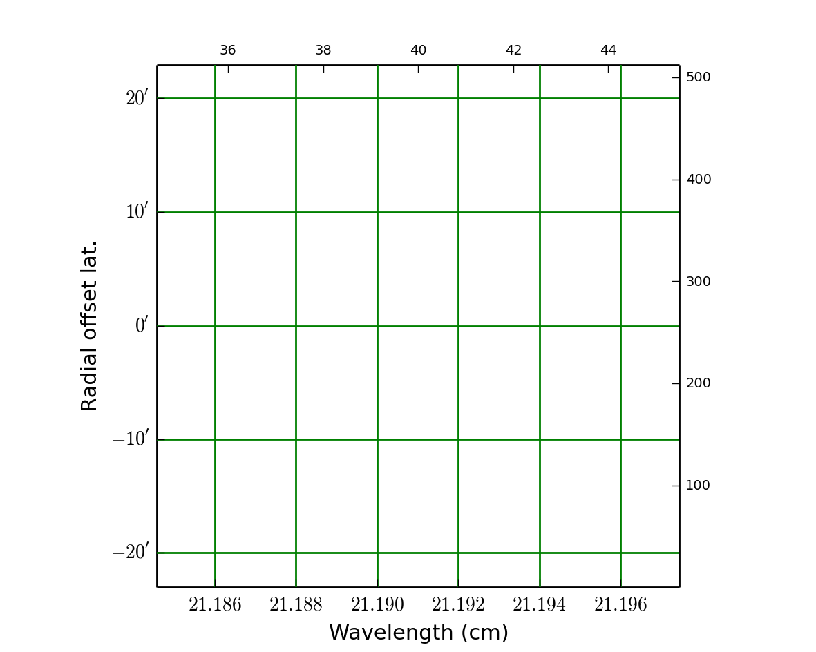
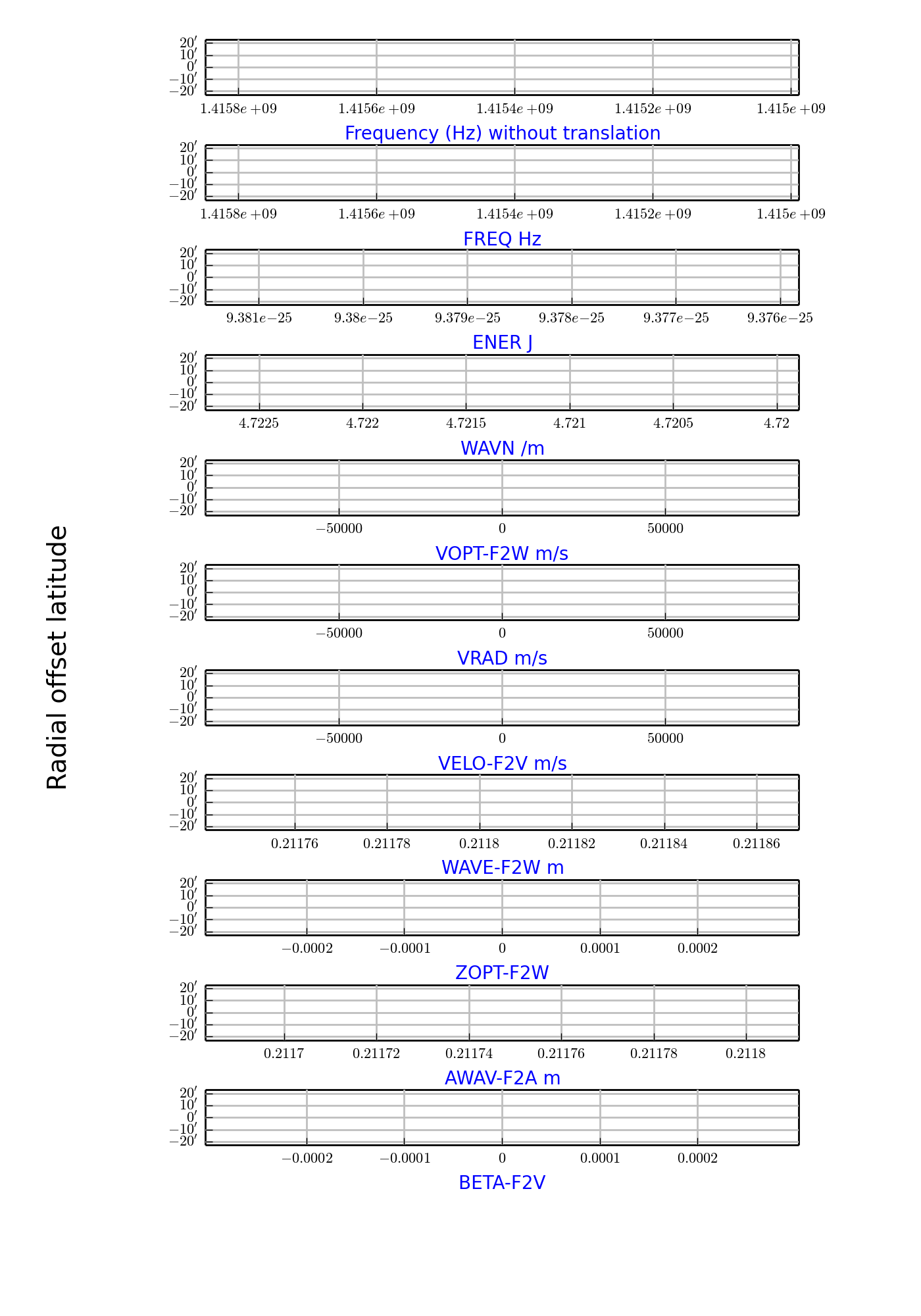
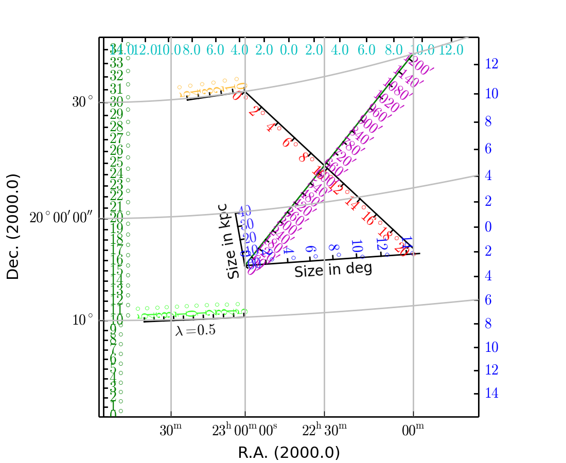
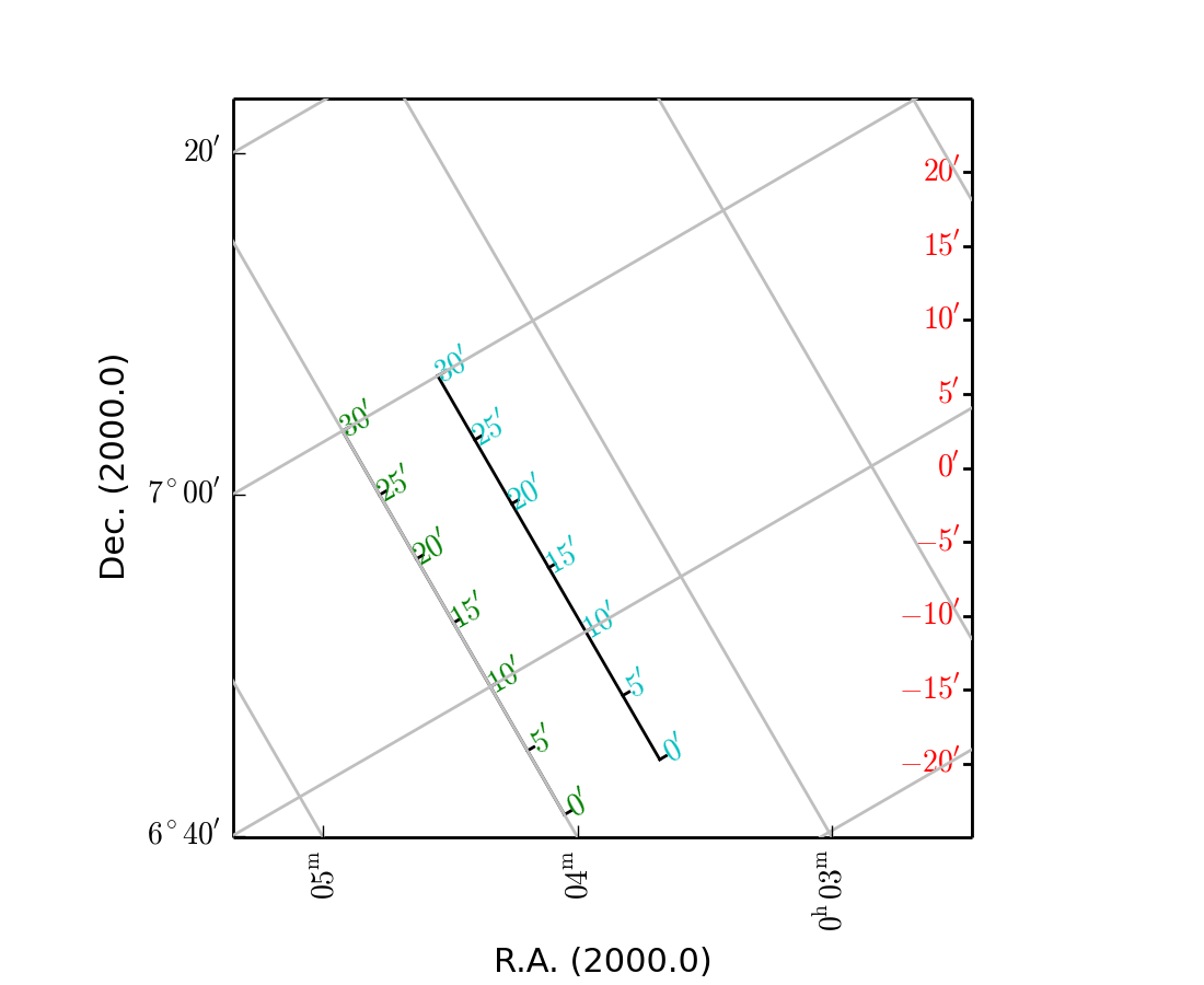
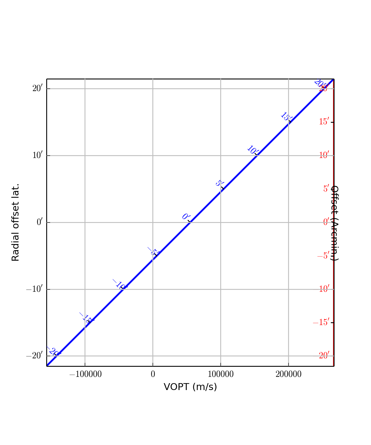
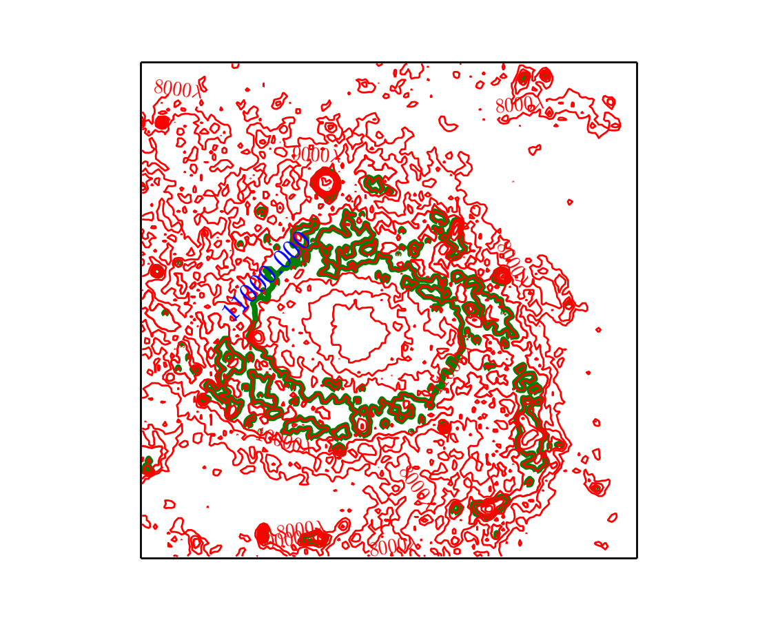
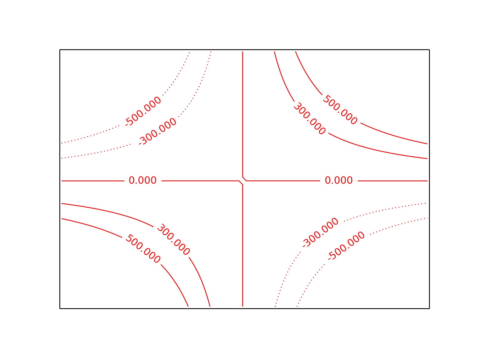
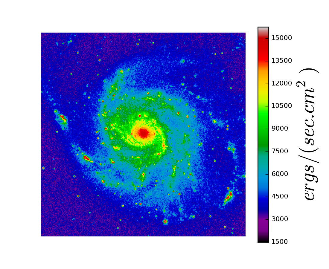
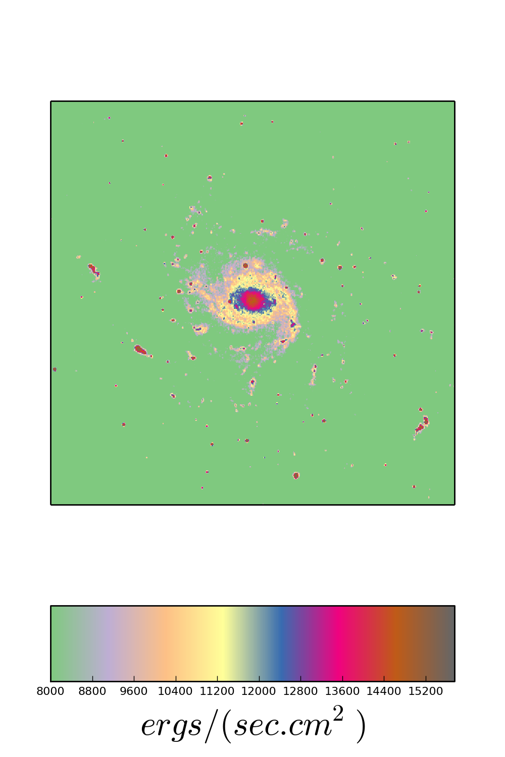
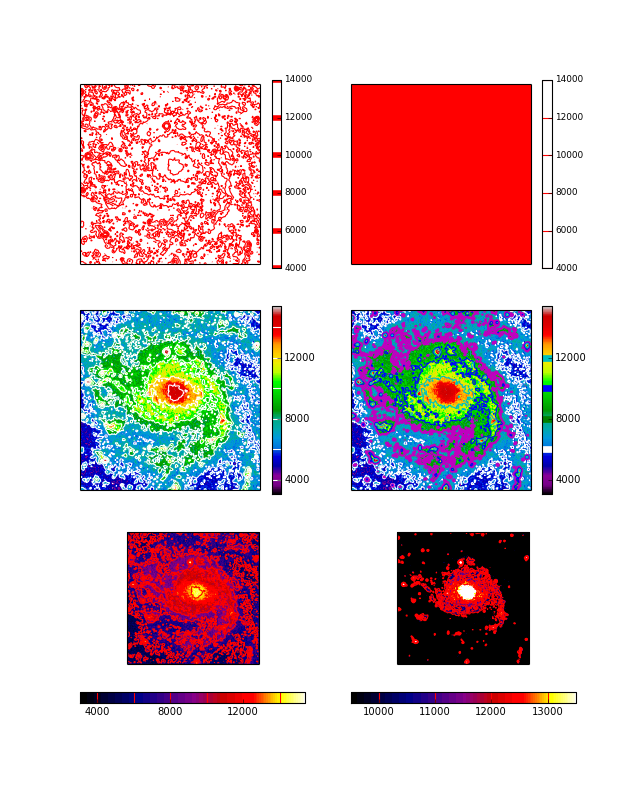
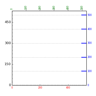
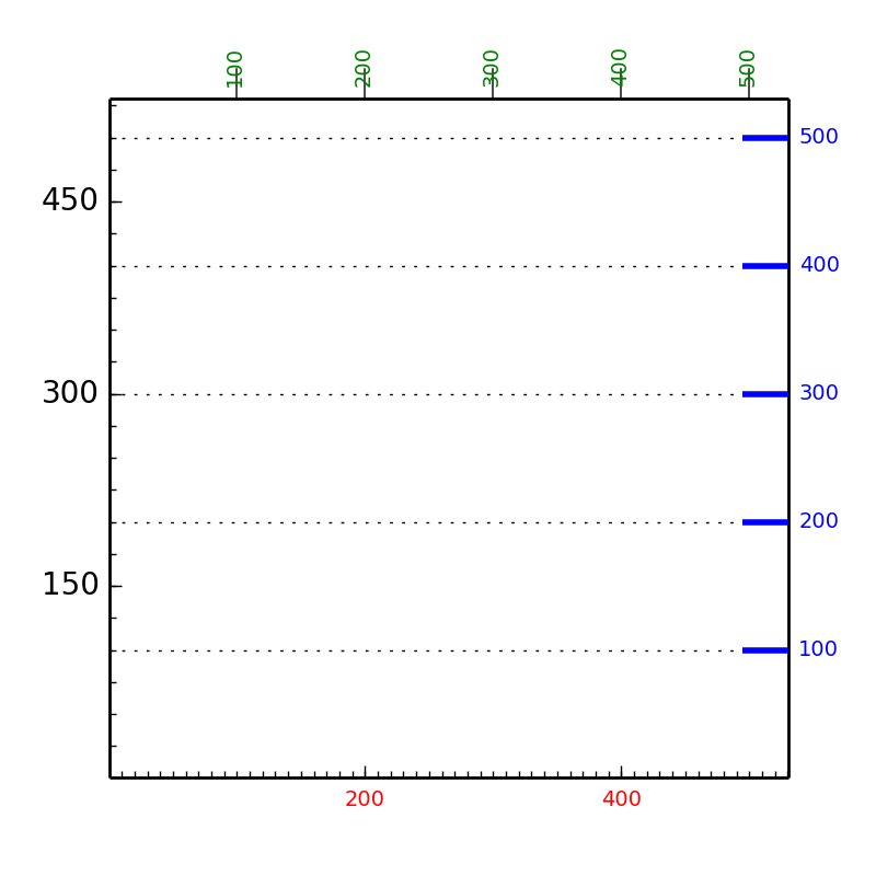
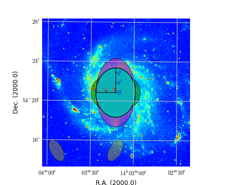
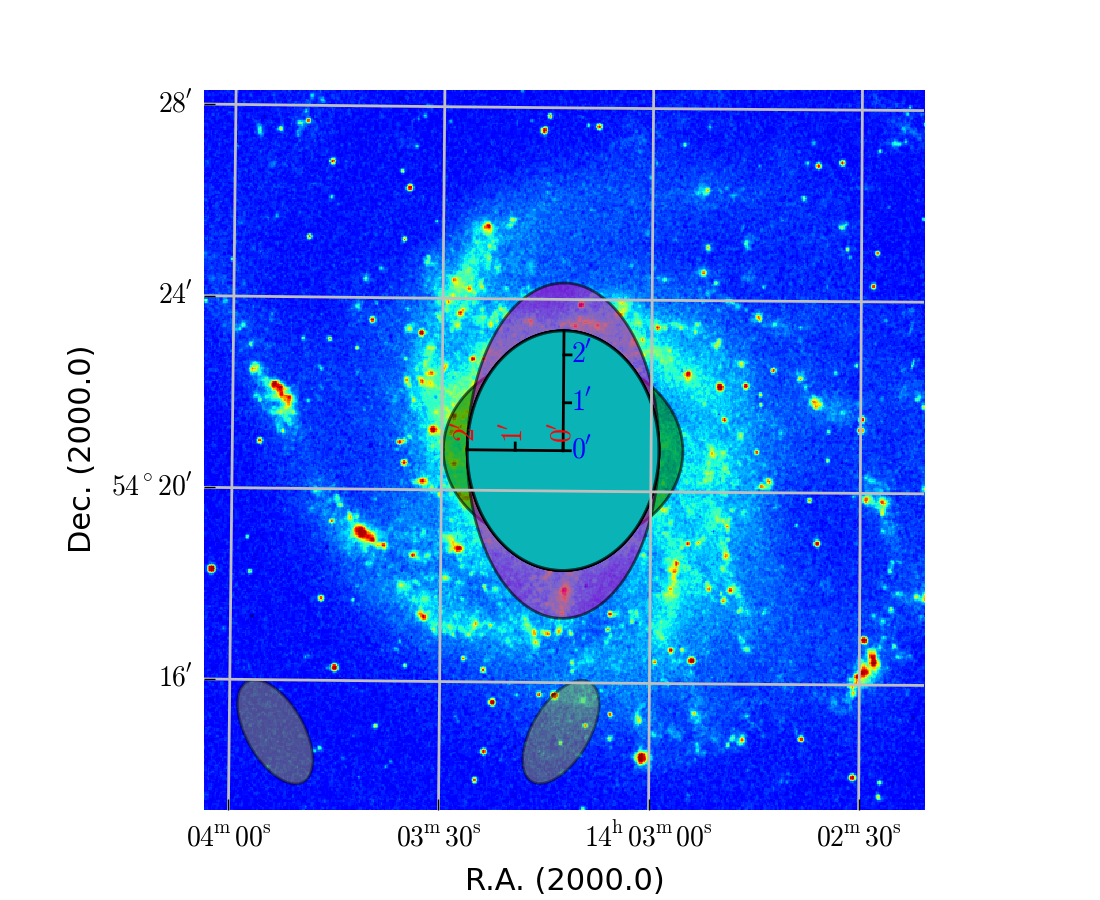
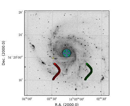
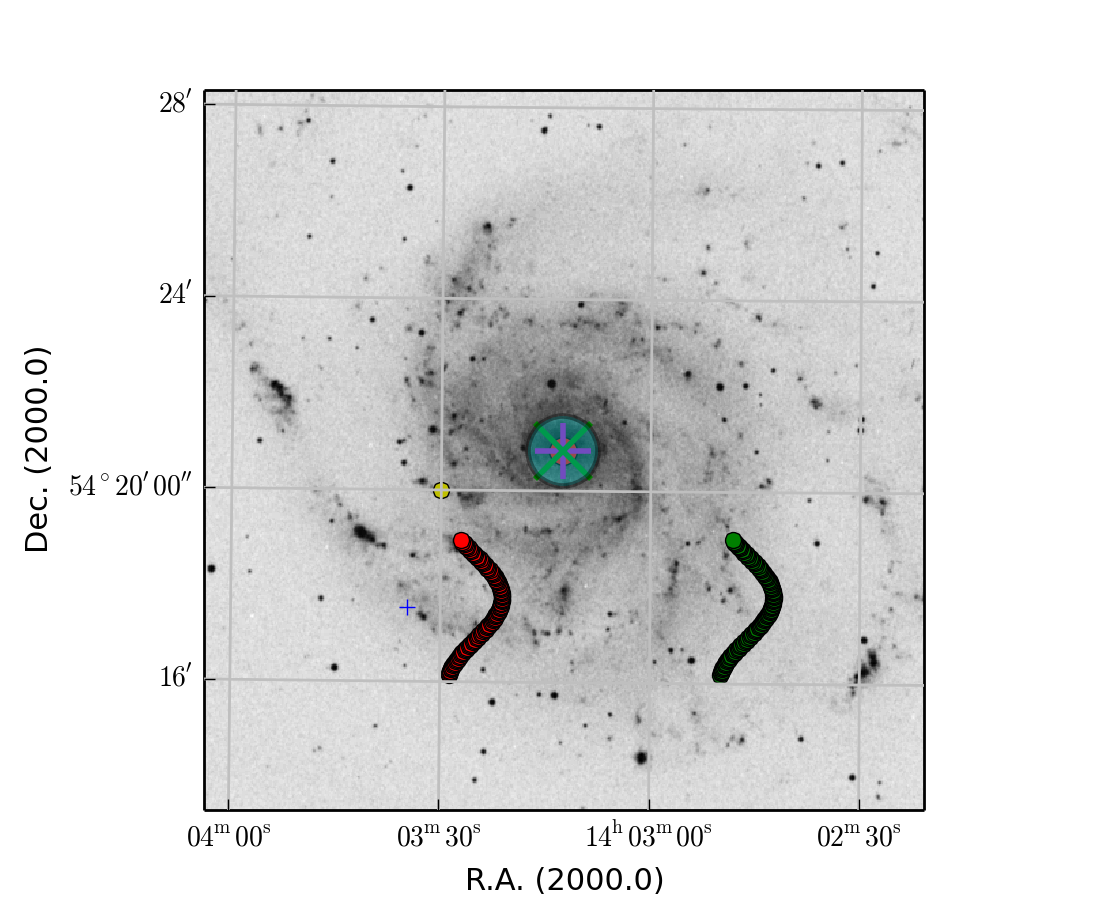
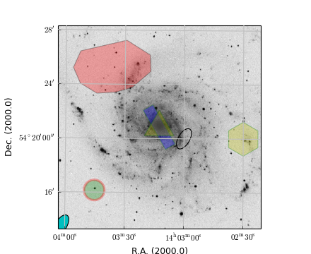
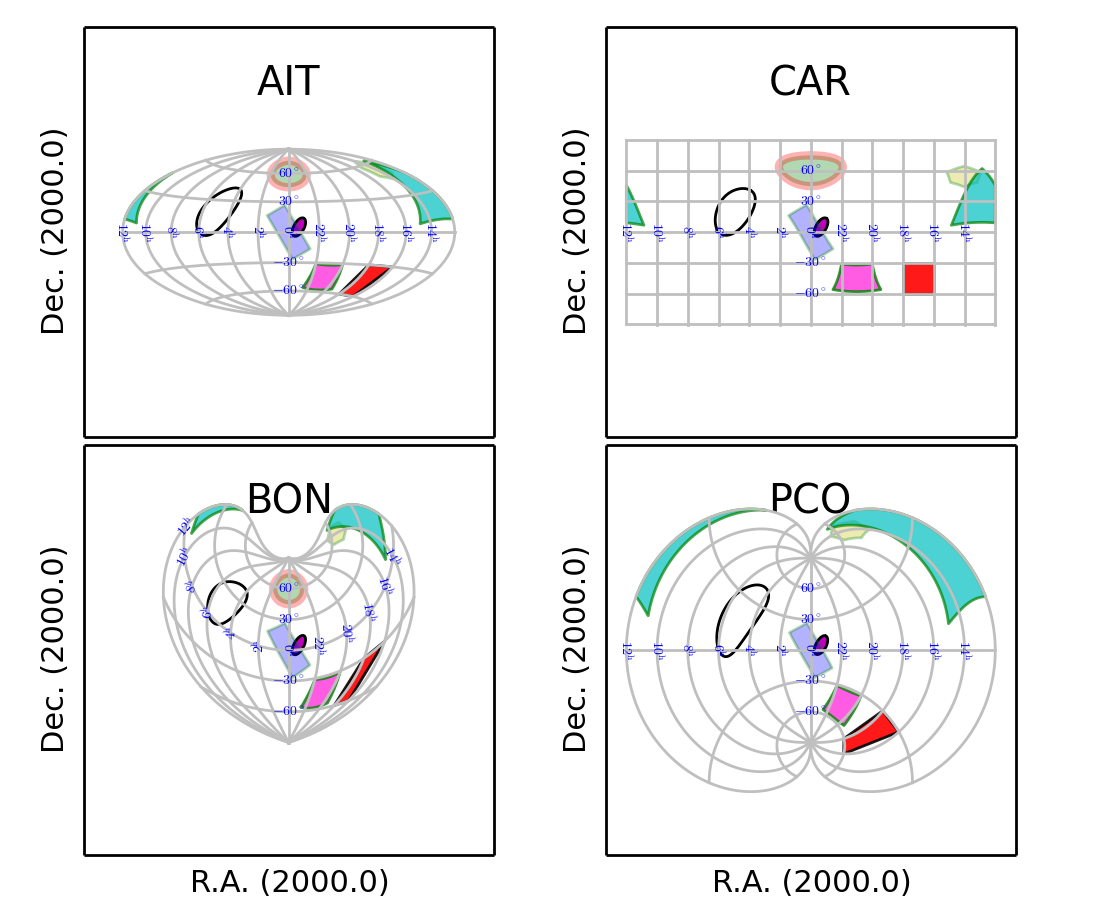
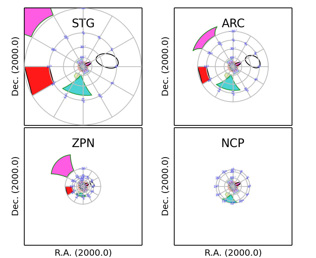
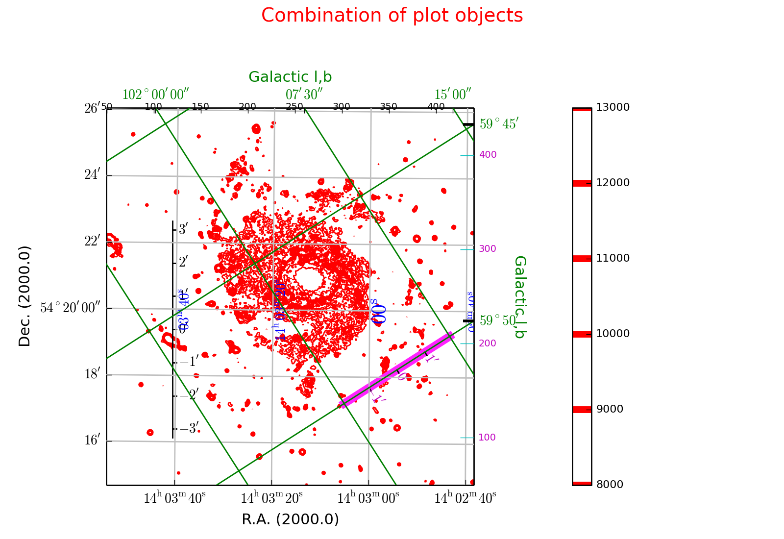
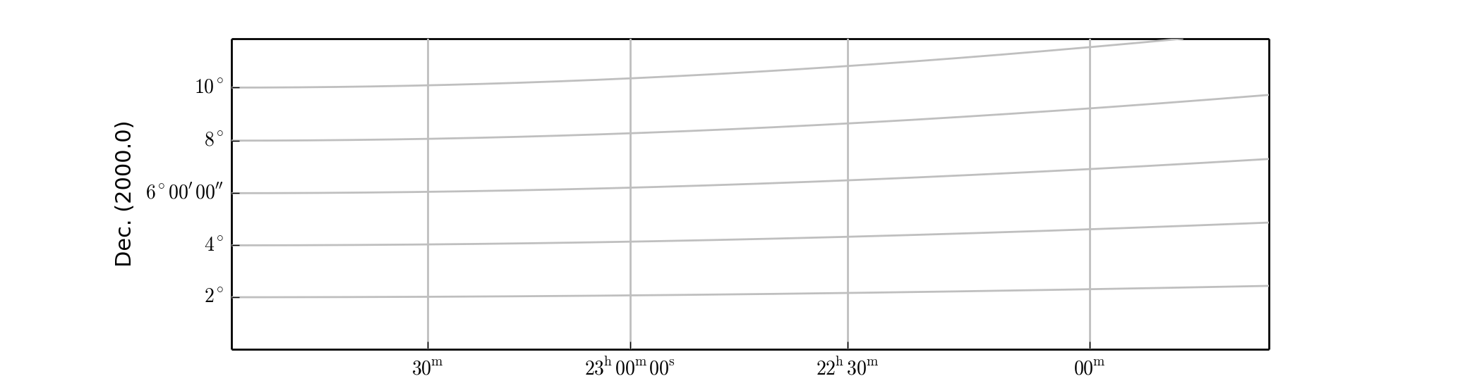
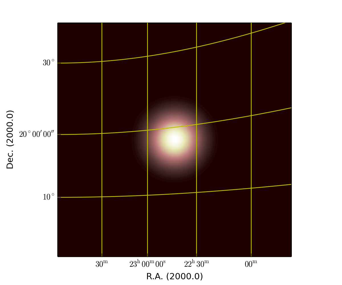
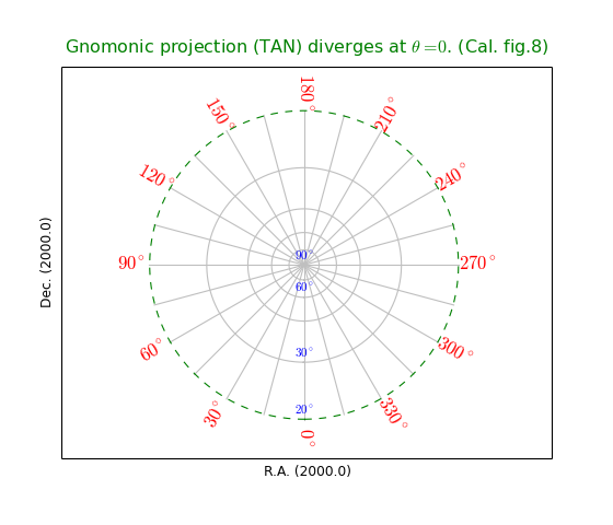
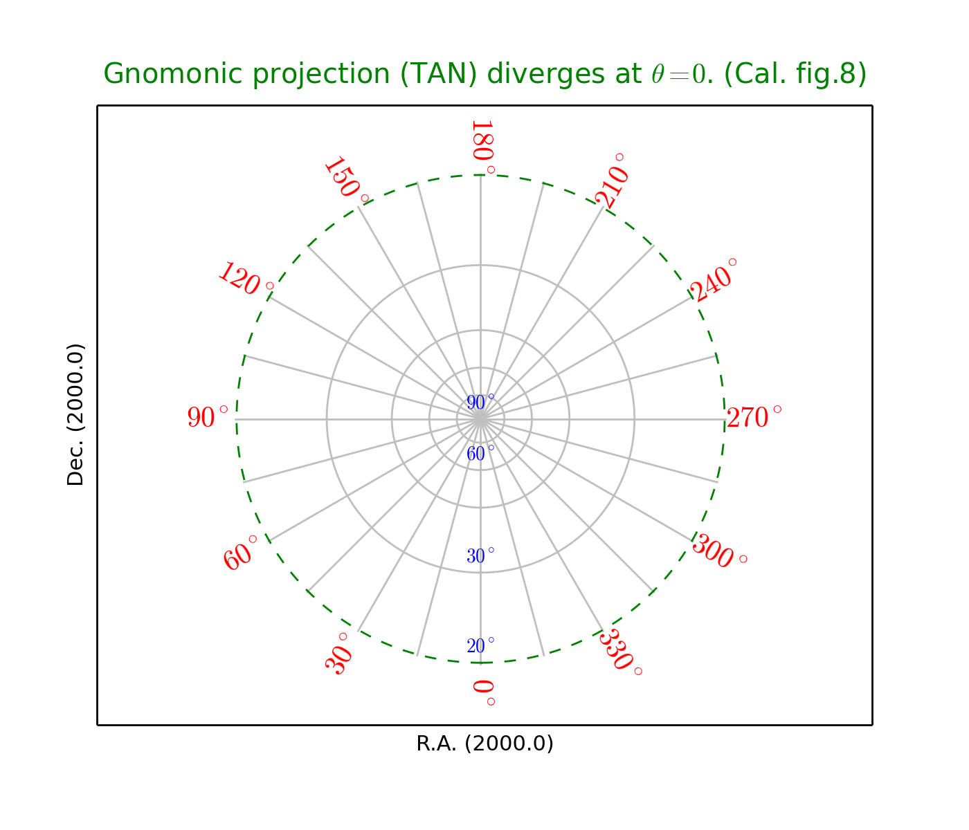
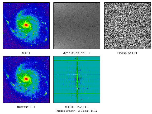
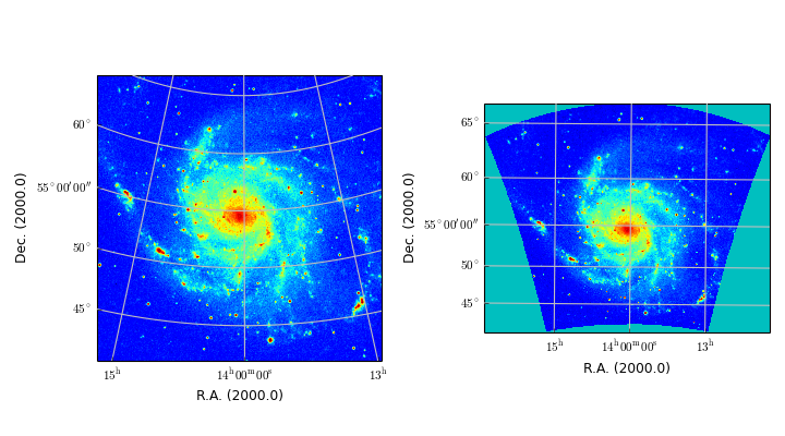
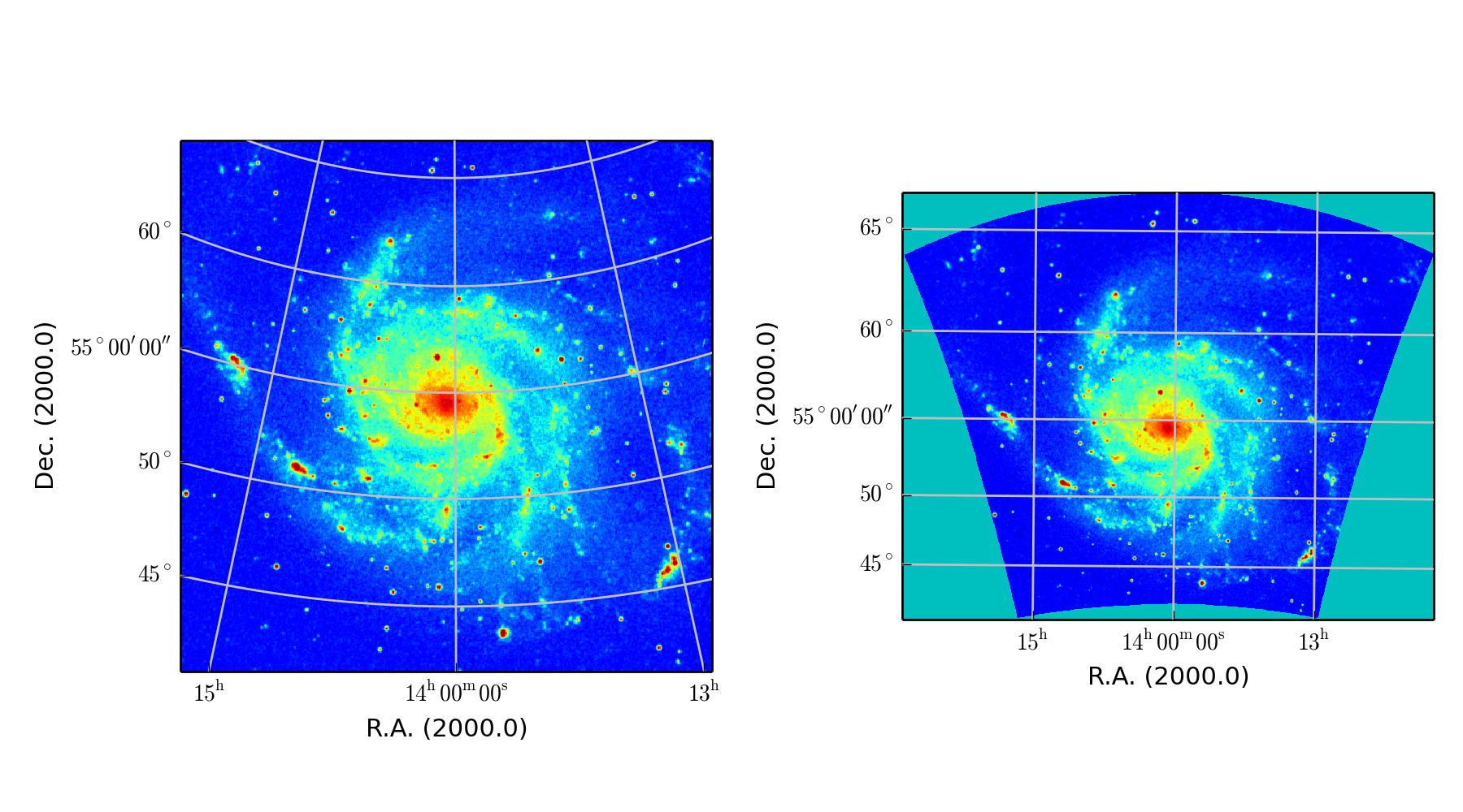
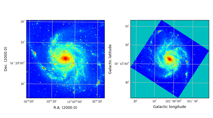
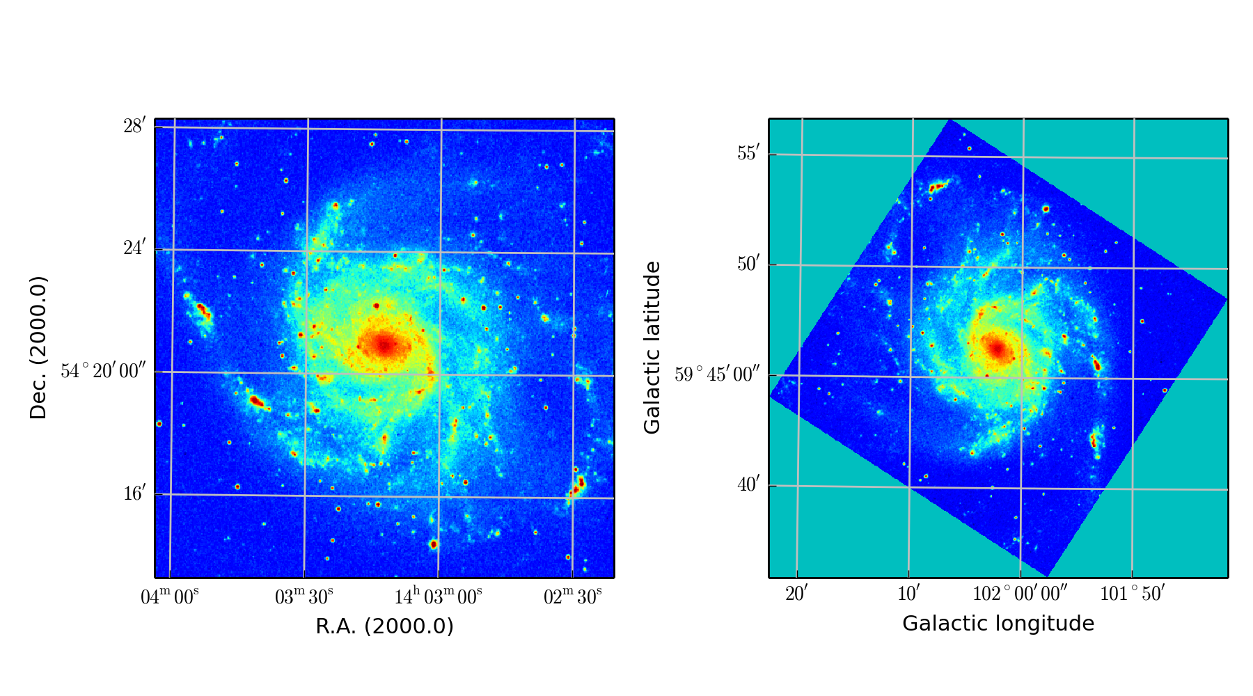
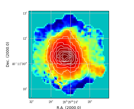
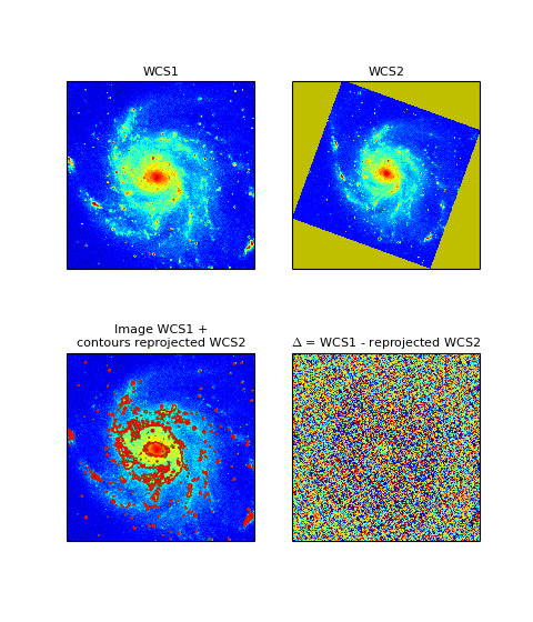
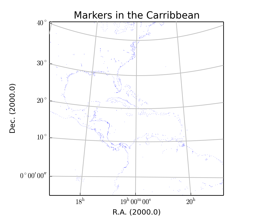
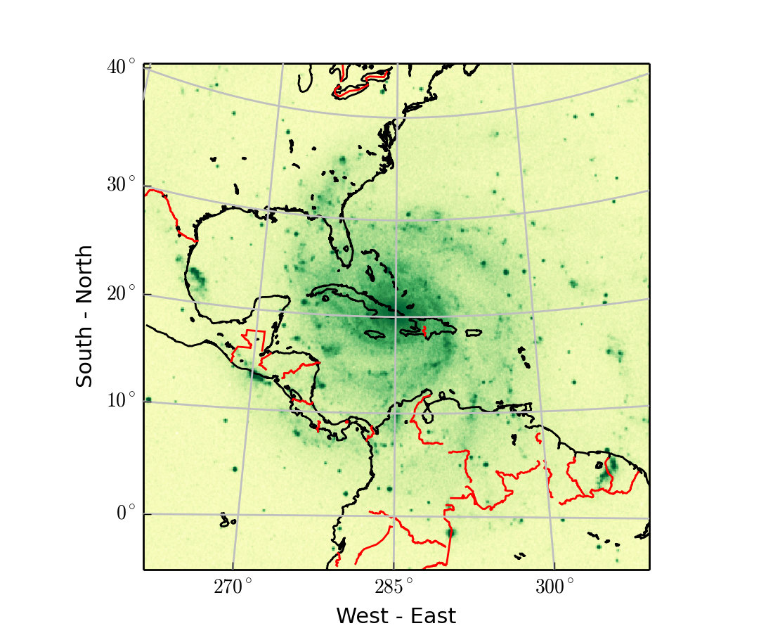
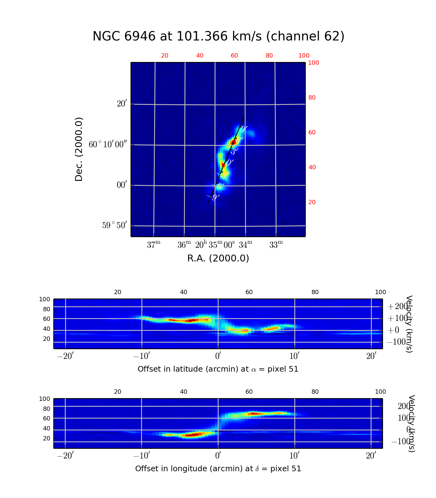
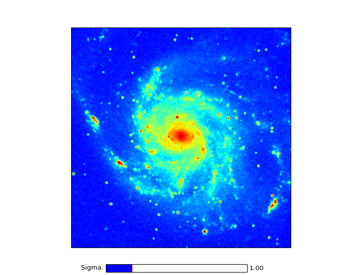
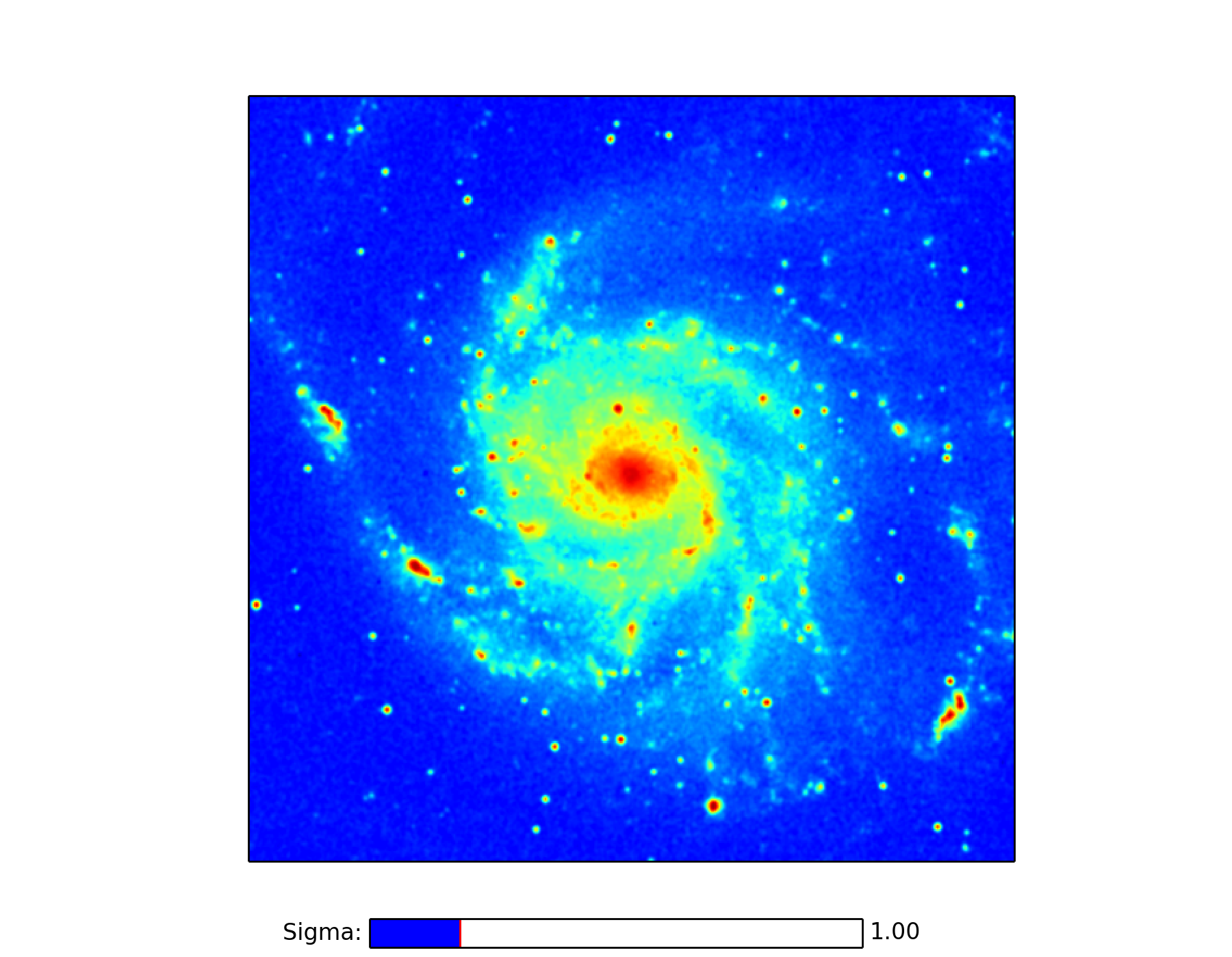
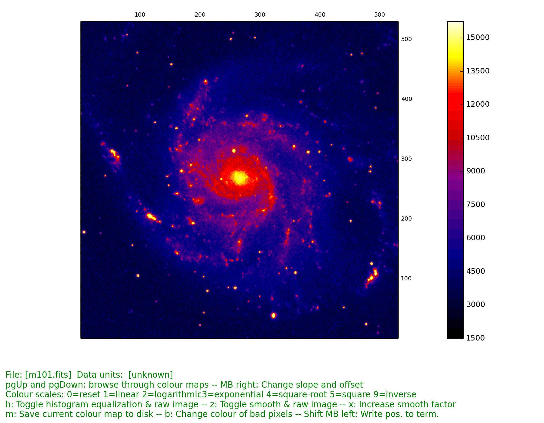