Kapteyn Institute Kapteyn Package

Module maputils

In the maputils tutorial we show many examples with Python code and figures to illustrate the functionality and flexibility of this module. The documentation below is restricted to the module’s classes and methods.

Introduction

One of the goals of the Kapteyn Package is to provide a user/programmer basic tools to make plots (with WCS annotation) of image data from FITS files. These tools are based on the functionality of PyFITS and Matplotlib. The methods from these packages are modified in maputils for an optimal support of inspection and presentation of astronomical image data with easy to write and usually very short Python scripts. To illustrate what can be done with this module, we list some steps you need in the process to create a hard copy of an image from a FITS file:

  • Open FITS file on disk or from a remote location (URL)
  • Specify in which header data unit the image data is stored
  • Specify the data slice for data sets with dimensions > 2
  • Specify the order of the image axes
  • Set the limits in pixels of both image axes
  • Set the sky system in which you want to plot wcs information.

Then for the display:

  • Plot the image or a mosaic of images in the correct aspect ratio
  • Plot (labeled) contours
  • Plot world coordinate labels along the image axes (basic routines in wcsgrat)
  • Plot coordinate graticules (basic routines in wcsgrat)
  • Interactively change color map and color limits
  • Read the position of features in a map and write these positions in your terminal.
  • Resize your plot canvas to get an optimal layout while preserving the aspect ratio.
  • Write the result to png or pdf (or another format from a list)

Of course there are many programs that can do this job some way or the other. But most probably no program does it exactly the way you want or the program does too much. Also many applications cannot be extended, at least not as simple as with the building blocks in maputils.

Module maputils is also very useful as a tool to extract and plot data slices from data sets with more than two axes. For example it can plot so called Position-Velocity maps from a radio interferometer data cube with channel maps. It can annotate these plots with the correct WCS annotation using information about the ‘missing’ spatial axis.

To facilitate the input of the correct data to open a FITS image, to specify the right data slice or to set the pixel limits for the image axes, we implemented also some helper functions. These functions are primitive (terminal based) but effective. You can replace them by enhanced versions, perhaps with a graphical user interface.

Here is an example of what you can expect. We have a three dimensional data set on disk called ngc6946.fits with axes RA, DEC and VELO. The program prompts the user to enter image properties like data limits, axes and axes order. The image below is a data slice in RA, DEC at VELO=50. We changed interactively the color map (keys page-up/page-down) and the color limits (pressing right mouse button while moving the mouse) and saved a hard copy on disk.

In the next code we use keyword parameter promptfie a number of times. Abbreviation ‘fie’ stands for Function Interactive Environment.

 1
 2
 3
 4
 5
 6
 7
 8
 9
10
11
12
13
14
15
16
17
18
19
20
21
22
23
24
25
26
27
#!/usr/bin/env python
from kapteyn import wcsgrat, maputils
from matplotlib import pylab as plt

   
# Create a maputils FITS object from a FITS file on disk
fitsobject = maputils.FITSimage(promptfie=maputils.prompt_fitsfile)
fitsobject.set_imageaxes(promptfie=maputils.prompt_imageaxes)
fitsobject.set_limits(promptfie=maputils.prompt_box)
fitsobject.set_skyout(promptfie=maputils.prompt_skyout)
clipmin, clipmax = maputils.prompt_dataminmax(fitsobject)
   
# Get connected to Matplotlib
fig = plt.figure()
frame = fig.add_subplot(1,1,1)

# Create an image to be used in Matplotlib
annim = fitsobject.Annotatedimage(frame, clipmin=clipmin, clipmax=clipmax)
annim.Image()
annim.Graticule()
annim.plot()

annim.interact_toolbarinfo()
annim.interact_imagecolors()
annim.interact_writepos()

plt.show()
_images/mu_introduction.png

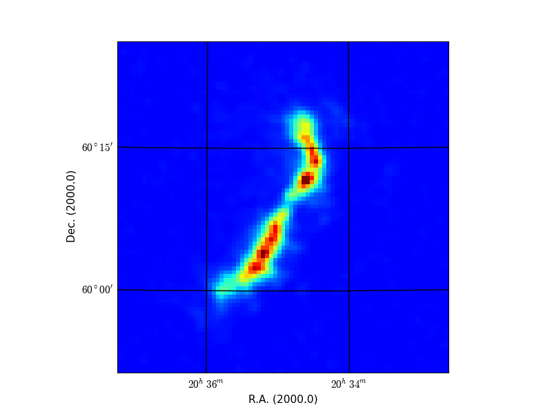
Image from FITS file with graticules and WCS labels

Module level data

cmlist

Object from class Colmaplist which has attribute colormaps which is a sorted list with names of colormaps. It has attributes:

  • colormaps – List with names of color lookup tables
  • cmap_default – Color map set by default to ‘jet’
Example:
 1
 2
 3
 4
 5
 6
 7
 8
 9
10
11
12
13
14
>>> from kapteyn import maputils
>>> print maputils.cmlist.colormaps
>>> cmap = raw_input("Enter name of a colormap: ")
['Accent', 'Blues', 'BrBG', 'BuGn', 'BuPu', 'Dark2',
'GnBu', 'Greens', 'Greys', 'OrRd', 'Oranges', 'PRGn',
'Paired', 'Pastel1', 'Pastel2', 'PiYG', 'PuBu', 'PuBuGn',
'PuOr', 'PuRd', 'Purples', 'RdBu', 'RdGy', 'RdPu',
'RdYlBu', 'RdYlGn', 'Reds', 'Set1', 'Set2', 'Set3',
'Spectral', 'YlGn', 'YlGnBu', 'YlOrBr', 'YlOrRd',
'autumn', 'binary', 'bone', 'cool', 'copper', 'flag',
'gist_earth', 'gist_gray', 'gist_heat', 'gist_ncar',
'gist_rainbow', 'gist_stern', 'gist_yarg', 'gray',
'hot', 'hsv', 'jet', 'pink', 'prism', 'spectral',
'spring', 'summer', 'winter']

Prompt functions

maputils.prompt_fitsfile(defaultfile=None, prompt=True, hnr=None, alter=None, memmap=None)

An external helper function for the FITSimage class to prompt a user to open the right Header and Data Unit (hdu) of a FITS file. A programmer can supply his/her own function of which the return value is a sequence containing the hdu list, the header unit number, the filename and a character for the alternate header.

Parameters:
  • defaultfile (String) – Name of FITS file on disk or url of FITS file on the internet. The syntax follows the standard described in the PyFITS documentation. See also the examples.
  • prompt (Boolean) – If False and a default file exists, then do not prompt for a file name. Open file and start checking HDU’s
  • hnr (Integer) – The number of the FITS header that you want to use. This function lists the hdu information and when hnr is not given, you will be prompted.
  • alter (Empty or a single character. Input is case insensitive.) – Selects an alternate header. Default is the standard header. Keywords in alternate headers end on a character A..Z
  • memmap (Boolean) – Set PyFITS memory mapping on/off. Let PyFITS set the default.
Prompts:
  1. Enter name of fits file ...... [a default]:

    Enter name of file on disk of valid url.

  2. Enter number of Header Data Unit ...... [0]:

    If a FITS file has more than one HDU, one must decide which HDU contains the required image data.

Returns:
  • hdulist - The HDU list and the user selected index of the wanted hdu from that list. The HDU list is returned so that it can be closed in the calling environment.
  • hnr - FITS header number. Usually the first header, i.e. hnr=0
  • fitsname - Name of the FITS file.
  • alter - A character that corresponds to an alternate header (with alternate WCS information e.g. a spectral translation).
Notes:

Examples:

Besides file names of files on disk, PyFITS allows url’s and gzipped files to retrieve FITS files e.g.:

http://www.atnf.csiro.au/people/mcalabre/data/WCS/1904-66_ZPN.fits.gz
maputils.prompt_imageaxes(fitsobj, axnum1=None, axnum2=None, slicepos=None)

Helper function for FITSimage class. It is a function that requires interaction with a user. Therefore we left it out of any class definition. so that it can be replaced by any other function that returns the position of the data slice in a FITS file.

It prompts the user for the names of the axes of the wanted image. For a 2D FITS data set there is nothing to ask, but for dimensions > 2, we should prompt the user to enter two image axes. Then also a list with pixel positions should be returned. These positions set the position of the data slice on the axes that do not belong to the image. Only with this information the right slice can be extracted.

The user is prompted in a loop until a correct input is given. If a spectral axis is part of the selected image then a second prompt is prepared for the input of the required spectral translation.

Parameters:
  • fitsobj (Instance of class FITSimage) – An object from class FITSimage. This prompt function derives useful attributes from this object such as the allowed spectral translations.
  • axnum1 (Integer [1, NAXIS]) – The axis number of the first (horizontal in terms of plot software) axis of the selected image which should be used as the default in the prompt. If None then the default is set to 1.
  • axnum2 (Integer [1, NAXIS]) – The axis number of the first (horizontal in terms of plot software) axis of the selected image which should be used as the default in the prompt. If None then the default is set to 1. If both axnum1 and axnum2 are specified then the image axis input prompt is skipped.
Prompts:
Name of the image axes:

Enter 2 axes from (list with allowed axis names) .... [default]:

e.g.: Enter 2 axes from (RA,DEC,VELO) .... [RA,DEC]:

The axis names can be abbreviated. A minimal match is applied.

Returns:

Tuple with three elements:

  • axnum1: Axis number of first image axis. Default or entered by a user.
  • axnum2: Axis number of second image axis. Default or entered by a user.
  • slicepos: A list with pixel positions. One pixel for each axis outside the image in the same order as the axes in the FITS header. These pixel positions are necessary to extract the right 2D data from FITS data with dimensions > 2.
Example:

Interactively set the axes of an image using a prompt function:

# Create a maputils FITSimage object from a FITS file on disk
fitsobject = maputils.FITSimage('rense.fits')
fitsobject.set_imageaxes(promptfie=maputils.prompt_imageaxes)
maputils.prompt_box(pxlim, pylim, axnameX, axnameY)

External helper function which returns the limits in pixels of the x- and y-axis. The input syntax is: xlo,xhi, ylo,yhi. For x and y the names of the image axes are substituted. Numbers can be separated by comma’s and or spaces. A number can also be specified with an expression e.g. 0, 10,  10/3, 100*numpy.pi. All these numbers are converted to integers.

Parameters:
  • pxlim (tuple with two integers) – Sequence of two numbers representing limits in pixels along the x axis as defined in the FITS file.
  • pylim (tuple with two integers) – Sequence of two numbers representing limits in pixels along the y axis as defined in the FITS file.
  • axnameX (String) – Name of image X-axis
  • axnameY (String) – Name of image Y-axis
Prompts:

Enter pixel limits in Xlo,Xhi, Ylo,Yhi ..... [xlo,xhi, ylo,yhi]:

The default should be the axis limits as defined in the FITS header in keywords NAXISn. In a real case this could look like:

Enter pixel limits in RAlo,RAhi, DEClo,DEChi ..... [1, 100, 1, 100]:

Returns:

Tuple with two elements pxlim, pylim (see parameter description)

Notes:

This function does not check if the limits are within the index range of the (FITS)image. This check is done in the FITSimage.set_limits() method of the FITSimage class.

Examples:

Use of this function as prompt function in the FITSimage.set_limits() method:

fitsobject = maputils.FITSimage('rense.fits')
fitsobject.set_imageaxes(1,2, slicepos=30) # Define image in cube
fitsobject.set_limits(promptfie=maputils.prompt_box)

This ‘box’ prompt needs four numbers. The first is the range in x and the second is the range in y. The input are pixel coordinates, e.g.:

>>>  0, 10   10/3, 100*numpy.pi

Note the mixed use of spaces and comma’s to separate the numbers. Note also the use of NumPy for mathematical functions. The numbers are truncated to integers.

maputils.prompt_spectrans(fitsobj)

Ask user to enter spectral translation if one of the axes is spectral.

Parameters:

fitsobj (Instance of class FITSimage) – An object from class FITSimage. From this object we derive the allowed spectral translations.

Prompts:

The spectral translation if one of the image axes is a spectral axis.

Enter number between 0 and N of spectral translation .... [native]:

N is the number of allowed translations minus 1. The default Native in this context implies that no translation is applied. All calculations are done in the spectral type given by FITS header item CTYPEn where n is the number of the spectral axis.

Returns:
  • spectrans - The selected spectral translation from a list with spectral translations that are allowed for the input object of class FITSimage. A spectral translation translates for example frequencies to velocities.
Example:
>>> fitsobject = maputils.FITSimage(promptfie=maputils.prompt_fitsfile)
>>> print fitsobject.str_spectrans()    # Print a list with options first
>>> fitsobject.set_spectrans(promptfie=maputils.prompt_spectrans)
maputils.prompt_skyout(fitsobj)

Ask user to enter the output sky system if the data is a spatial map.

Parameters:

fitsobj (Instance of class FITSimage) – An object from class FITSimage. This prompt function uses this object to get information about the axis numbers of the spatial axes in a data structure.

Returns:
  • skyout - The sky definition to which positions in the native system

    will be transformed.

Example:
>>> fitsobject = maputils.FITSimage(promptfie=maputils.prompt_fitsfile)
>>> fitsobject.set_skyout(promptfie=maputils.prompt_skyout)
maputils.prompt_dataminmax(fitsobj)
Ask user to enter one or two clip values. If one clip level is entered then in display routines the data below this value will be clipped. If a second level is entered, then all data values above this level will also be filtered.
Parameters:

fitsobj (Instance of class FITSimage) – An object from class FITSimage.

Returns:
  • clipmin, clipmax - Two values to set limits on the image value e.g. for color editing.
Example:
>>> fitsobject = maputils.FITSimage(promptfie=maputils.prompt_fitsfile)
>>> clipmin, clipmax = maputils.prompt_dataminmax(fitsobject)
>>> annim = fitsobject.Annotatedimage(frame, clipmin=clipmin, clipmax=clipmax)

Utility functions

maputils.fitsheader2dict(header, comment=True, history=True)

Transform a FITS header (read with PyFITS) into a Python dictionary. This is useful if one wants to iterate over all keys in the header. The PyFITS header is not iterable.

maputils.dist_on_sphere(l1, b1, l2, b2)

Formula for distance on sphere accurate over entire sphere (Vincenty, Thaddeus, 1975). Input and output are in degrees.

Parameters:
  • l1 (float) – Longitude of first location on sphere
  • b1 (float) – Latitude of first location on sphere
  • l2 (float) – Longitude of second location on sphere
  • b2 (float) – Latitude of second location on sphere
Examples:
>>> from kapteyn.maputils import dist_on_sphere
>>> print dist_on_sphere(0,0, 20,0)
    20.0
>>> print dist_on_sphere(0,30, 20,30)
    17.2983302106
maputils.showall()

Usually in a script with only one object of class maputils.Annotatedimage one plots this object, and its derived objects, with method maputils.Annotatedimage.plot(). Matplotlib must be instructed to do the real plotting with pyplot’s function show(). This function does this all.

Examples:
1
2
3
4
5
6
>>> im1 = f1.Annotatedimage(frame1)
>>> im1.Image()
>>> im1.Graticule()
>>> im2 = f2.Annotatedimage(frame2)
>>> im2.Image()
>>> maputils.showall()

Class FITSimage

class maputils.FITSimage(filespec=None, promptfie=None, prompt=True, hdunr=None, alter='', memmap=None, externalheader=None, externaldata=None, externalname='artificial', **parms)

This class extracts 2D image data from FITS files. It allows for external functions to prompt users for relevant input like the name of the FITS file, which header in that file should be used, the axis numbers of the image axes, the pixel limits and a spectral translation if one of the selected axes is a spectral axis. All the methods in this class that allow these external functions for prompting can also be used without these functions. Then one needs to know the properties of the FITS data beforehand.

Parameters:
  • filespec (String) – A default file either to open directly or to be used in a prompt as default file. This variable should have a value if no external function is used to prompt a user.
  • promptfie (Python function) – A user supplied function which should prompt a user for some data, opens the FITS file and returns the hdu list and a user selected index for the header from this hdu list. An example of a function supplied by maputils is function prompt_fitsfile()
  • hdunr (Integer) – A preset of the index of the header from the hdu list. If this variable is set then it should not prompted for in the user supplied function promptfie.
  • alter (Empty or a single character. Input is case insensitive.) – Selects an alternate header for the world coordinate system. Default is the standard header. Keywords in alternate headers end on a character A..Z
  • memmap (Boolean) – Set the memory mapping for PyFITS. The default is copied from the default in your version of PyFITS. If you want to be sure it is on then specify memmap=1
  • externalheader (Python dictionary) – If defined, then it is a header from an external source e.g. a user defined header.
  • externaldata (Numpy array) – If defined, then it is data from an external source e.g. user defined data or processed data in a numpy array. A user/programmer should check if the shape of the numpy array fits the sizes given in FITS keywords NAXISn.
  • parms (keyword arguments) – Extra parameters for PyFITS’s open() method, such as uint16, ignore_missing_end, checksum, see PyFITS documentation for their meaning.
Attributes:
filename

Name of the FITS file (read-only).

hdr

Header as read from the header (read-only).

naxis

Number of axes (read-only).

dat

The raw image data (not sliced, swapped or limited in range). The required sliced image data is stored in attribute boxdat. This is a read-only attribute.

axperm

Axis permutation array. These are the (FITS) axis numbers of your image x & y axis.

wcstypes

Type of the axes in this data. The order is the same as of the axes. The types ara strings and are derived from attribute wcstype of the Projection object. The types are: ‘lo’ is longitude axis. ‘la’ is latitude axis, ‘sp’ is spectral axis. ‘li’ is a linear axis. Appended to ‘li’ is an underscore and the ctype of that axis (e.g. ‘li_stokes’).

mixpix

The missing pixel if the image has only one spatial axis. The other world coordinate could be calculated with a so called mixed method which allows for one world coordinate and one pixel.

axisinfo

A list with FITSaxis objects. One for each axis. The index is an axis number (starting at 1).

slicepos

A list with positions on axes in the FITS file which do not belong to the required image.

pxlim

Axis limit in pixels. This is a tuple or list (xlo, xhi).

pylim

Axis limit in pixels. This is a tuple or list (xlo, xhi).

boxdat

The image data. Possibly sliced, axis swapped and limited in axis range.

imshape

Sizes of the 2D array in boxdat.

spectrans

A string that sets the spectra translation. If one uses the prompt function for the image axes, then you will get a list of possible translations for the spectral axis in your image.

proj

An object from wcs.Projection. This object is the result of the call: proj = wcs.Projection(self.hdr), so it is the Projection object that involves all the axes in the FITS header.

convproj

An object from wcs.Projection. This object is needed to be able to use methods toworld() and topixel() for the current image.

figsize

A suggested figure size (inches) in X and Y directions.

aspectratio

Plot a circle in world coordinates as a circle. That is, if the pixel size in the FITS header differs in X and Y, then correct the (plot) size of the pixels with value aspectratio so that features in an image have the correct sizes in longitude and latitude in degrees.

Notes:

The object is initialized with a default position for a data slice if the dimension of the FITS data is > 2. This position is either the value of CRPIX from the header or 1 if CRPIX is outside the range [1, NAXIS].

Values -inf and +inf in a dataset are replaced by NaN’s (not a number number). We know that Matplotlib’s methods have problems with these values, but these methods can deal with NaN’s.

Examples:

PyFITS allows URL’s to retrieve FITS files. It can also read gzipped files e.g.:

1
2
3
4
5
6
7
8
9
>>> f = 'http://www.atnf.csiro.au/people/mcalabre/data/WCS/1904-66_ZPN.fits.gz'
>>> fitsobject = maputils.FITSimage(f)
>>> print fitsobject.str_axisinfo()
Axis 1: RA---ZPN  from pixel 1 to   192
  {crpix=-183 crval=0 cdelt=-0.0666667 (Unknown)}
  {wcs type=longitude, wcs unit=deg}
Axis 2: DEC--ZPN  from pixel 1 to   192
  {crpix=22 crval=-90 cdelt=0.0666667 (Unknown)}
  {wcs type=latitude, wcs unit=deg}

Use Maputil’s prompt function prompt_fitsfile() to get user interaction for the FITS file specification.

>>> fitsobject = maputils.FITSimage(promptfie=maputils.prompt_fitsfile)
Methods:
set_imageaxes(axnr1=None, axnr2=None, slicepos=None, promptfie=None)

A FITS file can contain a data set of dimension n. If n < 2 we cannot display the data without more information. If n == 2 the data axes are those in the FITS file, Their numbers are 1 and 2. If n > 2 then we have to know the numbers of those axes that are part of the image. For the other axes we need to know a pixel position so that we are able to extract a data slice.

Attribute dat is then always a 2D array.

Parameters:
  • axnr1 (Integer or String) – Axis number of first image axis (X-axis). If it is a string, then the number of the first axis which matches is returned. The string match is minimal and case insensitive.
  • axnr2 (Integer or String) – Axis number of second image axis (Y-axis). If it is a string, then the number of the first axis which matches is returned. The string match is minimal and case insensitive.
  • slicepos (Integer or sequence of integers) – list with pixel positions on axes outside the image at which an image is extracted from the data set. Applies only to data sets with dimensions > 2. The length of the list must be equal to the number of axes in the data set that are not part of the image.
  • spectrans (Integer) – The spectral translation to convert between different spectral types if one of the image axes has spectral type.
  • promptfie – A Function that for in an Interactive Environment (fie), supplied by the user, that can prompt a user to enter the values for axnr1, axnr2 and slicepos. An example of a function supplied by maputils is function prompt_imageaxes()
Raises:
Exception

One axis number is missing and no prompt function is given!

Exception

Missing positions on axes outside image! – Somehow there are not enough elements in parameter slicepos. One should supply as many pixel positions as there are axes in the FITS data that do not belong to the selected image.

Exception

Cannot find a matching axis for the spatial axis! – The matching spatial axis for one of the image axes could not be found in the FITS header. It will not be possible to get useful world coordinates for the spatial axis in your image.

Modifies attributes:
axisinfo

A dictionary with objects from class FITSaxis. One object for each axis. The dictionary keys are the axis numbers. See also second example at method FITSaxis.printattr().

allowedtrans
A list with strings representing the spectral translations that are possible for the current image axis selection.
spectrans

The selected spectral translation

slicepos

One or a list with integers that represent pixel positions on axes in the data set that do not belong to the image. At these position, a slice with image data is extracted.

map

Image data from the selected FITS file. It is always a 2D data slice and its size can be found in attribute imshape.

imshape

The shape of the array map.

mixpix

Images with only one spatial axis, need another spatial axis to produces useful world coordinates. This attribute is extracted from the relevant axis in attribute slicepos.

convproj

An object from class Projection as defined in wcs.

axperm

The axis numbers corresponding with the X-axis and Y-axis in the image.

Note:

The aspect ratio is reset (to None) after each call to this method.

Examples:

Set the image axes explicitly:

>>> fitsobject = maputils.FITSimage('rense.fits')
>>> fitsobject.set_imageaxes(1,2, slicepos=30)

Set the images axes in interaction with the user using a prompt function:

>>> fitsobject = maputils.FITSimage('rense.fits')
>>> fitsobject.set_imageaxes(promptfie=maputils.prompt_imageaxes)

Enter (part of) the axis names. Note the minimal matching and case insensitivity.

>>> fitsobject = maputils.FITSimage('rense.fits')
>>> fitsobject.set_imageaxes('ra','d', slicepos=30)
set_limits(pxlim=None, pylim=None, promptfie=None)

This method sets the image box. That is, it sets the limits of the image axes in pixels. This can be a useful feature if one knows which part of an image contains the interesting data.

Parameters:
  • pxlim (Tuple with two integers) – Two integer numbers which should not be smaller than 1 and not bigger than the header value NAXISn, where n represents the x axis.
  • pylim (Tuple with two integers) – Two integer numbers which should not be smaller than 1 and not bigger than the header value NAXISn, where n represents the y axis.
  • promptfie (Python function) – An external function with parameters pxlim, pylim, axnameX, and axnameY which are used to compose a prompt. If a function is given then there is no need to enter pxlim and pylim. The prompt function must return (new) values for pxlim and pylim. An example of a function supplied by maputils is function prompt_box()
Examples:

Ask user to enter limits with prompt function prompt_box()

>>> fitsobject = maputils.FITSimage('rense.fits')
>>> fitsobject.set_imageaxes(1,2, slicepos=30) # Define image in cube
>>> fitsobject.set_limits(promptfie=maputils.prompt_box)
set_spectrans(spectrans=None, promptfie=None)

Set spectral translation or ask user to enter a spectral translation if one of the axes in the current FITSimage is spectral.

Parameters:
  • spectrans (String) – A spectral translation e.g. to convert frequencies to optical velocities.
  • promptfie (A Python function without parameters. It returns a string with the spectral translation. An example of a function supplied by maputils is function prompt_spectrans()) – A function, supplied by the user, that can prompt a user to enter a sky definition.
Examples:

Set a spectral translation using 1) a prompt function, 2) a spectral translation for which we don’t know the code for the conversion algorithm and 3) set the translation explicitly:

>>> fitsobject.set_spectrans(promptfie=maputils.prompt_spectrans)
>>> fitsobject.set_spectrans(spectrans="VOPT-???")
>>> fitsobject.set_spectrans(spectrans="VOPT-V2W")
set_skyout(skyout=None, promptfie=None)

Set the output sky definition. Mouse positions and coordinate labels will correspond to the selected definition. The method will only work if both axes are spatial axes.

Parameters:
  • skyout (A single value or tuple.) – The output sky definition for sky system, reference system, equinox and date of observation. For the syntax of a sky definition see the description at celestial.skymatrix()
  • promptfie (A Python function without parameters. It returns the sky definition. An example of a function supplied by maputils is function prompt_skyout()) – A function, supplied by the user, that can prompt a user to enter a sky definition.
Notes:

The method sets an output system only for data with two spatial axes. For XV maps the output sky system is always the same as the native system.

Annotatedimage(frame=None, **kwargs)

This method couples the data slice that represents an image to a Matplotlib Axes object (parameter frame). It returns an object from class Annotatedimage which has only attributes relevant for Matplotlib.

Parameters:
  • frame (A Matplotlib Axes instance) – Plot the current image in this Matplotlib Axes object. If omitted, a default frame will be set using Matplotlib’s method add_subplot()
  • kwargs (Python keyword arguments) –

    These parameters are keyword arguments for the constructor of Annotatedimage. All of them get a default value in this routine. The ones for which it can be useful to change are:

    • skyout: The sky definition for graticule and world coordinates
    • spectrans: The spectral translation for the spectral axis
    • aspect: The aspect ratio of the pixels
    • basename: A name for a file on disk e.g. to store a color lut
    • cmap: A color map
    • blankcolor: The color of bad pixels,
    • clipmin: Scale colors between image values clipmin and clipmax
    • clipmax: Scale colors between image values clipmin and clipmax
    • gridmode: Set modus of str2pos() to pixels or grids
Attributes:

See documentation at Annotatedimage

Returns:

An object from class Annotatedimage

Examples:
>>> f = maputils.FITSimage("ngc6946.fits")
>>> f.set_imageaxes(1, 3, slicepos=51)
>>> annim = f.Annotatedimage()

or:

 1
 2
 3
 4
 5
 6
 7
 8
 9
10
11
from kapteyn import maputils
from matplotlib import pyplot as plt

f = maputils.FITSimage("m101.fits")
fig = plt.figure()
frame = fig.add_subplot(1,1,1)
annim = f.Annotatedimage(frame)
annim.Image()
annim.Graticule()
annim.plot()
plt.show()
get_pixelaspectratio()

Return the aspect ratio of the pixels in the current data structure defined by the two selected axes. The aspect ratio is defined as pixel height / pixel width.

Example:
>>> fitsobject = maputils.FITSimage('m101.fits')
>>> print fitsobject.get_pixelaspectratio()
1.0002571958
Note:

If a header has only a cd matrix and no values for CDELT, then these values are set to 1. This gives an aspect ratio of 1.

get_figsize(xsize=None, ysize=None, cm=False)

Usually a user will set the figure size manually with Matplotlib’s figure(figsize=...) construction. For many plots this is a waste of white space around the plot. This can be improved by taking the aspect ratio into account and adding some extra space for labels and titles. For aspect ratios far from 1.0 the number of pixels in x and y are taken into account.

A handy feature is that you can enter the two values in centimeters if you set the flag cm to True.

If you have a plot which is higher than its width and you want to fit in on a A4 page then use:

>>> f = maputils.FITSimage(externalheader=header)
>>> figsize = f.get_figsize(ysize=21, cm=True)
>>> fig = plt.figure(figsize=figsize)
>>> frame = fig.add_subplot(1,1,1)
str_header()

Print the meta information from the selected header. Omit items of type HISTORY. It prints both real FITS headers and headers given by a dictionary.

Returns:

A string with the header keywords

Examples:

If you think a user needs more information from the header than can be provided with method str_axisinfo() it can be useful to display the contents of the selected FITS header. This is the entire header and not a selected alternate header.

 1
 2
 3
 4
 5
 6
 7
 8
 9
10
11
12
13
14
15
16
>>> from kapteyn import maputils
>>> fitsobject = maputils.FITSimage('rense.fits')
>>> print fitsobject.str_header()
SIMPLE  =                    T / SIMPLE FITS FORMAT
BITPIX  =                  -32 / NUMBER OF BITS PER PIXEL
NAXIS   =                    3 / NUMBER OF AXES
NAXIS1  =                  100 / LENGTH OF AXIS
NAXIS2  =                  100 / LENGTH OF AXIS
NAXIS3  =                  101 / LENGTH OF AXIS
BLOCKED =                    T / TAPE MAY BE BLOCKED
CDELT1  =  -7.165998823000E-03 / PRIMARY PIXEL SEPARATION
CRPIX1  =   5.100000000000E+01 / PRIMARY REFERENCE PIXEL
CRVAL1  =  -5.128208479590E+01 / PRIMARY REFERENCE VALUE
CTYPE1  = 'RA---NCP          ' / PRIMARY AXIS NAME
CUNIT1  = 'DEGREE            ' / PRIMARY AXIS UNITS
etc. etc.
str_axisinfo(axnum=None, long=False)

For each axis in the FITS header, return a string with the data related to the World Coordinate System (WCS).

Parameters:
  • axnum (None, Integer or list with Integers) – A list with axis numbers for which one wants to print information. These axis numbers are FITS numbers i.e. in range [1,NAXIS]. To display information about the two image axes one should use attribute maputils.FITSimage.axperm as in the second example below.
  • long (Boolean) – If True then more verbose information is printed.
Returns:

A string with WCS information for each axis in axnum.

Examples:

Print useful header information after the input of the FITS file and just before the specification of the image axes:

 1
 2
 3
 4
 5
 6
 7
 8
 9
10
11
12
>>> from kapteyn import maputils
>>> fitsobject = maputils.FITSimage('rense.fits')
>>> print fitsobject.str_axisinfo()
Axis 1: RA---NCP  from pixel 1 to   100
  {crpix=51 crval=-51.2821 cdelt=-0.007166 (DEGREE)}
  {wcs type=longitude, wcs unit=deg}
Axis 2: DEC--NCP  from pixel 1 to   100
  {crpix=51 crval=60.1539 cdelt=0.007166 (DEGREE)}
  {wcs type=latitude, wcs unit=deg}
Axis 3: VELO-HEL  from pixel 1 to   101
  {crpix=-20 crval=-243 cdelt=4200 (km/s)}
  {wcs type=spectral, wcs unit=m/s}

Print extended information for the two image axes only:

>>> print str_axisinfo(axnum=fitsobject.axperm, long=True)
Notes:

For axis numbers outside the range of existing axes in the FITS file, nothing will be printed. No exception will be raised.

str_wcsinfo()

Compose a string with information about the data related to the current World Coordinate System (WCS) (e.g. which axes are longitude, latitude or spectral axes)

Returns:

String with WCS information for the current Projection object.

Examples:

Print information related to the world coordinate system:

 1
 2
 3
 4
 5
 6
 7
 8
 9
10
11
12
>>> print fitsobject.str_wcsinfo()
Current sky system:                 Equatorial
reference system:                   ICRS
Output sky system:                  Equatorial
Output reference system:            ICRS
projection's epoch:                 J2000.0
Date of observation from DATE-OBS:  2002-04-04T09:42:42.1
Date of observation from MJD-OBS:   None
Axis number longitude axis:         1
Axis number latitude axis:          2
Axis number spectral axis:          None
Allowed spectral translations:      None
str_spectrans()

Compose a string with the possible spectral translations for this data.

Returns:

String with information about the allowed spectral translations for the current Projection object.

Examples:

Print allowed spectral translations:

>>> print fitsobject.str_spectrans()
get_dataminmax(box=False)

Get minimum and maximum value of data in entire data structure defined by the current FITS header or in a slice. These values can be important if you want to compare different images from the same source (e.g. channel maps in a radio data cube).

Parameters:

box (Boolean) – Find min, max in data or if set to True in data slice (with limits).

Returns:

min, max, two floating point numbers representing the minimum and maximum data value in data units of the header (BUNIT).

Note:

We assume here that the data is read when a FITSobject was created. Then the data is filtered and the -inf, inf values are replaced by NaN’s.

Example:

Note the difference between the min, max of the entire data or the min, max of the slice (limited by a box):

1
2
3
4
5
fitsobj = maputils.FITSimage('ngc6946.fits')
vmin, vmax = fitsobj.get_dataminmax()
for i, ch in enumerate(channels):
   fitsobj.set_imageaxes(lonaxnum, lataxnum, slicepos=ch)
   print "Min, max in this channel: ", fitsobj.get_dataminmax(box=True)
slice2world(skyout=None, spectra=None, userunits=None)

Given the pixel coordinates of a slice, return the world coordinates of these pixel positions and their units. For example in a 3-D radio cube with axes RA-DEC-FREQ one can have several RA-DEC images as function of FREQ. This FREQ is given in pixels coordinates in attribute slicepos. The world coordinates are calculated using the Projection object which is also an attribute.

Parameters:
  • skyout (String or tuple representing sky definition) – Set current projection object in new output sky mode
  • spectra (String) – Use this spectral translation for the output world coordinates
  • userunits (String) – A sequence of units as the user wants to have it appear in the slice info string. The order of these units must be equal to the order of the axes outside the slice/subset. Both the world coordinates and the units are adjusted.
Returns:

A tuple with two elements: world and units. Element world is either an empty list or a list with one or more world coordinates. The number of coordinates is equal to the number of axes in a data set that do not belong to the extracted data which can be a slice. For each world coordinate there is a unit in element units.

Note:

This method first calculates a complete set of world coordinates. Where it did not define a slice position, it takes the header value CRPIXn. So if a map is defined with only one spatial axes and the missing spatial axis is found in slicepos than we have two matching pixel coordinates for which we can calculate world coordinates. So by definition, if a slice is a function of a spatial coordinate, then its world coordinate is found by using the matching pixel coordinate which, in case of a spatial map, corresponds to the projection center.

Example:
>>> vel, uni = fitsobj.slice2world(spectra="VOPT-???")
>>> velinfo = "ch%d = %.1f km/s" % (ch, vel[0]/1000.0)

or: >>> vel, uni = fitsobj.slice2world(spectra=”VOPT-???”, userunits=”km/s”)

header2classic()

If a header contains PC or CD elements, and not all the ‘classic’ elements for a WCS then a number of FITS readers could have a problem if they don’t recognize a PC and CD matrix. What can be done is to derive the missing header items, CDELTn and CROTA from these headers and add them to the header.

What is a ‘classic’ FITS header?

(See also http://fits.gsfc.nasa.gov/fits_standard.html) For the transformation between pixel coordinates and world coordinates, FITS supports three conventions. First some definitions:

An intermediate pixel coordinate \(q_i\) is calculated from a pixel coordinates \(p\) with:

\[q_i = \sum_{j=1}^N m_{ij}(p_j-r_j)\]

Rj are the pixel coordinate elements of a reference point (FITS header item CRPIXj), j is an index for the pixel axis and i for the world axis The matrix \(m_{ij}\) must be non-singular and its dimension is NxN where N is the number of world coordinate axes (given by FITS header item NAXIS).

The conversion of \(q_i\) to intermediate world coordinate \(x_i\) is a scale \(s_i\):

\[x_i = s_i q_i\]

Formalism 1 (PC keywords)

Formalism 1 encodes \(m_{ij}\) in so called PCi_j keywords and scale factor \(s_i\) are the values of the CDELTi keywords from the FITS header.

It is obvious that the value of CDELT should not be 0.0.

Formalism 2 (CD keywords)

If the matrix and scaling are combined we get for the intermediate WORLD COORDINATE \(x_i\):

\[x_i = \sum_{j=1}^N (s_i m_{ij})(p_j-r_j)\]

FITS keywords CDi_j encodes the product \(s_i m_{ij}\). The units of \(x_i\) are given by FITS keyword CTYPEi.

Formalism 3 (Classic)

This is the oldest but now deprecated formalism. It uses CDELTi for the scaling and CROTAn for a rotation of the image plane. n is associated with the latitude axis so often one sees CROTA2 in the header if the latitude axis is the second axis in the dataset

Following the FITS standard, a number of rules is set:

  1. CDELT and CROTA may co-exist with the CDi_j keywords but must be ignored if an application supports the CD formalism.
  2. CROTAn must not occur with PCi_j keywords
  3. CRPIXj defaults to 0.0
  4. CDELT defaults to 1.0
  5. CROTA defaults to 0.0
  6. PCi_j defaults to 1 if i==j and to 0 otherwise. The matrix must not be singular
  7. CDi_j defaults to 0.0. The matrix must not be singular.
  8. CDi_j and PCi_j must not appear together in a header.

Alternate WCS axis descriptions

A World Coordinate System (WCS) can be described by an alternative set of keywords. For this keywords a character in the range [A..Z] is appended. In our software we made the assumption that the primary description contains all the necessary information to derive a ‘classic’ header and therefore we will ignore alternate header descriptions.

Conversion to a formalism 3 (‘classic’) header

Many FITS readers from the past are not upgraded to process FITS files with headers written using formalism 1 or 2. The purpose of this application is to convert a FITS file to a file that can be read and interpreted by old FITS readers. For GIPSY we require FITS headers to be written using formalism 3. If keywords are missing, they will be derived and a comment will be inserted about the keyword not being an original keyword.

The method that converts the header, tries to process it first with WCSLIB (tools to interpret the world coordinate system as described in a FITS header). If this fails, then we are sure that the header is incorrect and we cannot proceed. One should use a FITS tool like ‘fv’ (the Interactive FITS File Editor from Nasa) to repair the header.

The conversion process starts with exploring the spatial part of the header. It knows which axes are spatial and it reads the corresponding keywords (CDELTi, CROTAn, CDi_j, PCi_j and PC00i_00j (old format for PC elements). If there is no CD or PC matrix, then the conversion routine returns the unaltered original header. If it finds a PC matrix and no CD matrix then the header should contain CDELT keywords. With the values of these keywords we create a CD matrix:

\[\begin{split}\begin{bmatrix}cd_{11} & cd_{12}\\ cd_{21} & cd_{22}\end{bmatrix} = \begin{bmatrix}cdelt_1 & 0\\ 0 & cdelt_2 \end{bmatrix} \begin{bmatrix}pc_{11} & pc_{12}\\ pc_{21} & pc_{22}\end{bmatrix}\end{split}\]

Notes:

  • We replaced notation i_j by ij so cd11 == CD1_1
  • For the moment we restricted the problem to the 2 dim. spatial case because that is what we need to retrieve a value for CROTA, the rotation of the image.)
  • We assumed that the PC matrix did not represent transposed axes as in:
\[\begin{split}PC = \begin{bmatrix}0 & 1 & 0\\ 0 & 0 & 1\\ 1 & 0 & 0 \end{bmatrix}\end{split}\]

If cd12 == 0.0 and cd12 == 0.0 then CROTA is obviously 0. There is no rotation and CDELT1 = cd11, CDELT2 = cd22

If one or both values of cd12, cd21 is not zero then we expect a value for CROTA unequal to zero and/or skew.

We calculate the scaling parameters CDELT with:

CDELT1 = sqrt(cd11*cd11+cd21*cd21)
CDELT2 = sqrt(cd12*cd12+cd22*cd22)

The determinant of the matrix is:

det = cd11*cd22 - cd12*cd21

This value cannot be 0 because we required that the matrix is non-singular. Further we distinguish two situations: a determinant < 0 and a determinant > 0 (zero was already excluded). Then we derive two rotations. If these are equal, the image is not skewed. If they are not equal, we derive the rotation from the average of the two calculated angles. As a measure of skew, we calculated the difference between the two rotation angles. Here is a piece of the actual code:

1
2
3
4
5
6
7
8
9
sign = 1.0
if det < 0.0:
   cdeltlon_cd = -cdeltlon_cd
   sign = -1.0
rot1_cd = atan2(-cd21, sign*cd11)
rot2_cd = atan2(sign*cd12, cd22)
rot_av = (rot1_cd+rot2_cd)/2.0
crota_cd = degrees(rot_av)
skew = degrees(abs(rot1_cd-rot2_cd))

New values of CDELT and CROTA will be inserted in the new ‘classic’ header only if they were not part of the original header.

The process continues with non spatial axes. For these axes we cannot derive a rotation. We only need to find a CDELTi if for axis i no value could be found in the header. If this value cannot be derived from the a CD matrix (usually with diagonal element CDi_i) then the default 1.0 is assumed. Note that there will be a warning about this in the comment string for the corresponding keyword in the new ‘classic’ FITS header.

Finally there is some cleaning up. First all CD/PC elements are removed for all the axes in the data set. Second, some unwanted keywords are removed. The current list is: [“XTENSION”, “EXTNAME”, “EXTEND”]

See also: Calabretta & Greisen: ‘Representations of celestial coordinates in FITS’, section 6

Parameters:

- – No parameters

Returns:

A tuple with three elements:

  • hdr - A modified copy of the current header. The CD and PC elements are removed.
  • skew - Difference between the two calculated rotation angles If this number is bigger then say 0.001 then there is considerable skew in the data. One should reproject the data so that it fits a non skewed version with only a CROTA in the header
  • hdrchanged - A list with keywords the are changed when a ‘classic’ header is required.
Notes:

This method is tested with FITS files:

  • With classic header
  • With only CD matrix
  • With only PC matrix
  • With PC and CD matrix
  • With CD matrix and NAXIS > 2
  • With sample files with skew
Example:
1
2
3
4
5
6
7
8
9
from kapteyn import maputils, wcs
import pyfits
         
Basefits = maputils.FITSimage(promptfie=maputils.prompt_fitsfile)
newheader, skew, hdrchanged = Basefits.header2classic()
if len(hdrchanged):
   print newheader
if skew != 0.0:
   print "found skew:", skew
reproject_to(reprojobj=None, pxlim_dst=None, pylim_dst=None, plimlo=None, plimhi=None, interpol_dict=None, rotation=None, insertspatial=None, **fitskeys)

The current FITSimage object must contain a number of spatial maps. This method then reprojects these maps so that they conform to the input header.

Imagine an image and a second image of which you want to overlay contours on the first one. Then this method uses the current data to reproject to the input header and you will end up with a new FITSimage object which has the spatial properties of the input header and the reprojected data of the current FITSimage object.

Also more complicated data structures can be used. Assume you have a data cube with axes RA, Dec and Freq. Then this method will reproject all its spatial subsets to the spatial properties of the input header.

The current FITSimage object tries to keep as much of its original FITS keywords. Only those related to spatial data are copied from the input header. The size of the spatial map can be limited or extended. The axes that are not spatial are unaltered.

The spatial information for both data structures are extracted from the headers so there is no need to specify the spatial parts of the data structures.

The image that is reprojected can be limited in size with parameters pxlim_dst and pylim_dst. If the input is a FITSimage object, then these parameters (pxlim_dst and pylim_dst) are copied from the axes lengths set with method set_limits() for that FITSimage object.

Parameters:
  • reprojobj (Python dictionary or PyFITS header. Or a maputils.FITSimage object) –
    • The header which provides the new information to reproject to. The size of the reprojected map is either copied from the NAXIS keywords in the header or entered with parameters pxlim_dst and pylim_dst. The reprojections are done for all spatial maps in the current FITSimage object or for a selection entered with parameters plimlo and plimhi (see examples).
    • The FITSimage object from which relevant information is extracted like the header and the new sizes of the spatial axes which otherwise should have been provided in parameters pxlim_dst and pylim_dst. The reprojection is restricted to one spatial map and its slice information is copied from the current FITSimage. This option is selected if you want to overlay e.g. contours from the current FITSimage data onto data from another WCS.
    • If None, then the current header is used. Modifications to this header are done with keyword arguments.
  • pxlim_dst (Tuple of integers) – Limits in pixels for the reprojected box.
  • plimlo (Integer or tuple of integers) – One or more pixel coordinates corresponding to axes outside the spatial map in order as found in the header ‘reprojobj’. The values set the lower limits of the axes. There is no need to specify all limits but the order is important.
  • plimhi (Integer or tuple of integers) – The same as plimhi, but now for the upper limits.
  • interpol_dict (Python dictionary) –

    This parameter is a dictionary with parameters for the interpolation routine which is used to reproject data. The interpolation routine is based on SciPy’s map_coordinates. The most important parameters with the maputils defaults are:

    order : Integer, optional

    The order of the spline interpolation, default is 1. The order has to be in the range 0-5.

    mode : String, optional

    Points outside the boundaries of the input are filled according to the given mode (‘constant’, ‘nearest’, ‘reflect’ or ‘wrap’). Default is ‘constant’.

    cval : scalar, optional

    Value used for points outside the boundaries of the input if mode=’constant’. Default is numpy.NaN

  • rotation (Floating point number or None) – Sets a rotation angle. If this method encounters this keyword, it will create a so called ‘classic’ header. That is a header without CD or PC elements. Then the rotation angle of the current spatial map is only given by FITS keyword CROTAn. The value of rotation is added to CROTAn to create a new value which is inserted in the new header. Note that values for CROTAn in the fitskeys parameter list overwrite this calculated value.
  • insertspatial (Boolean) – If True, then replace spatial part of current header by spatial part of new (destination) header. Assume you start with a data cube with a number of spatial maps as function of frequency (the third axis in the data set). If you use the header of another FITS file as the definition of a new world coordinate system, then it could be that this header represents a two dimensional data set. This is not an incompatible set because we only require a description of the spatial part. To keep the description of the original three dimensional structure we insert the new spatial(only) information into the current header. The default then is insertspatial=True. In other cases where we use the original header as the base header, one just inserts new values and there is no need to set insert something, so then the default is insertspatial=False. A user can change the default. This can be useful. For example in the maputils tutorial we have a script mu_reproj2classic.py where we use the header of a FITS file to make some changes and use the changed header as an external header to re-project to. The default then is insertspatial=True, but the external header is already a complete header, so there is no need to insert something.
  • fitskeys (Python keyword arguments.) – Parameters containing FITS keywords and values which are written in the reprojection header.
Examples:

-Set limits for axes outside the spatial map. Assume a data structure with axes RA-DEC-FREQ-STOKES for which the RA-DEC part is reprojected to a set RA’-DEC’-FREQ-STOKES. The ranges for FREQ and STOKES set the number of spatial maps in this data structure. One can limit these ranges with plimlo and plimhi.

  • plimlo=(20,2), plimhi=(40,2)

    we restrict the reprojections for spatial maps at frequencies 20 to 40 at one position on the STOKES axis (at pixel coordinate 2).

  • plimlo=(None,2), plimhi=(None,2)

    If one wants to reproject all the maps at all frequencies but only for STOKES=2 and 3 then use: plimlo=(None,2) and plimhi=(None,2) where None implies no limits.

  • plimlo=40

    No plimhi is entered. Then there are no upper limits. Only one value (40) is entered so this must represent the FREQ axis at pixel coordinate 40. It represents all spatial maps from FREQ pixel coordinate 40 to the end of the FREQ range, repeated for all pixels on the STOKES axis.

  • plimlo=(55,1), plimhi=(55,1)

    This reprojects just one map at FREQ pixel coordinate 55 and STOKES pixel coordinate 1. This enables a user/programmer to extract one spatial map, reproject it and write it as a single map to a FITS file while no information about the FREQ and STOKES axes is lost. The dimensionality of the new data remains 4 but the length of the ‘repeat axes’ is 1.

Note that if the data structure was represented by axes FREQ-RA-STOKES-DEC then the examples above are still valid because these set the limits on the repeat axes FREQ and POL whatever the position of these axes in the data structure.

-Use and modify the current header to change the data. The example shows how to rotate an image and display the result.

 1
 2
 3
 4
 5
 6
 7
 8
 9
10
11
12
13
Basefits = maputils.FITSimage("m101.fits")
Rotfits = Basefits.reproject_to(rotation=40.0,
                              naxis1=800, naxis2=800,
                              crpix1=400, crpix2=400)

# If copy on disk required:
# Rotfits.writetofits("m10rot.fits", clobber=True, append=False)

annim = Rotfits.Annotatedimage()
annim.Image()
annim.Graticule()
annim.interact_toolbarinfo()
maputils.showall()

-Use an external header and change keywords in that header before the re-projection:

>>> Rotfits = Basefits.reproject_to(externalheader,
                                    naxis1=800, naxis2=800,
                                    crpix1=400, crpix2=400)

-Use the FITS file’s own header. Change it and use it as an external header

 1
 2
 3
 4
 5
 6
 7
 8
 9
10
11
12
from kapteyn import maputils, wcs

Basefits = maputils.FITSimage("m101.fits")
classicheader, skew, hdrchanged = Basefits.header2classic()

lat = Basefits.proj.lataxnum
key = "CROTA%d"%lat
classicheader[key] = 0.0 # New value for CROTA
Basefits.reproject_to(classicheader, insertspatial=False)
fnew = maputils.FITSimage(externalheader=classicheader,
                          externaldata=Basefits.dat)
fnew.writetofits("classic.fits", clobber=True, append=False)
Tests:
  1. The first test was a reprojection of data of map1 to the spatial header of map2. One should observe that the result of the reprojection (reproj) has its spatial structure from map2 and its non spatial structure (i.e. the repeat axes) from map1. Note that the order of longitude, latitude in map1 is swapped in map2.

    map1: CTYPE: RA - POL - FREQ - DEC NAXIS 35 5 16 41

    map2: CTYPE: DEC - POL - FREQ - RA NAXIS 36 4 17 30

    reproj = map1.reproject_to(map2)

    reproj: CTYPE: RA - POL - FREQ - DEC NAXIS 36 5 16 30

  2. Tested with values for the repeat axes

  3. Tested with values for the output box

  4. Tested with a new CTYPE (GLON-TAN, GLAT-TAN) and new CRVAL

Note

If you want to align an image with the direction of the north, then the value of CROTAn (e.g. CROTA2) should be set to zero. To ensure that the data will be rotated, use parameter rotation with a dummy value so that the header used for the re-projection is a ‘classic’ header:

e.g.:

>>> Rotfits = Basefits.reproject_to(rotation=0.0, crota2=0.0)
Todo: If CTYPE’s change, then also LONPOLE and LATPOLE
should change

Warning

Values for CROTAn in parameter fitskeys overwrite values previously set with keyword rotation.

Warning

Changing values of CROTAn will not always result in a rotated image. If the world coordinate system was defined using CD or PC elements, then changing CROTAn will only add the keyword but it is never read because CD & PC transformations have precedence.

writetofits(filename=None, comment=True, history=True, bitpix=None, bzero=None, bscale=None, blank=None, clobber=False, append=False, extname='')

This method copies current data and current header to a FITS file on disk. This is useful if either header or data comes from an external source. If no file name is entered then a file name will be composed using current date and time of writing. The name then start with ‘FITS’.

Parameters:
  • filename (String) – Name of new file on disk. If omitted the default name is ‘FITS’ followed by a date and a time (in hours, minutes seconds).
  • comment (Boolean) – If you do not want to copy comments, set parameter to False
  • history (Boolean) – If you do not want to copy history, set parameter to False
  • bitpix (Integer) – Write FITS data in another format (8, 16, 32, -32, -64). If no bitpix is entered then -32 is assumed. Parameters bzero, bscale and blank are ignored then.
  • bzero (Float) – Offset in scaled data. If bitpix is not equal to -32 and the values for bscale and bzero are None, then the data is scaled between the minimum and maximum data values. For this scaling the method scale() from PyFITS is used with option='minmax'. However PyFITS 1.3 generates an error due to a bug.
  • bscale (Float) – Scale factor for scaled data. If bitpix is not equal to -32 and the values for bscale and bzero are None, then the data is scaled between the minimum and maximum data values. For this scaling the method scale() from PyFITS is used with option='minmax'. However PyFITS 1.3 generates an error due to a bug.
  • blank (Float/Integer) – Value that represents a blank. Usually only for scaled data.
  • clobber (Boolean) – If a file on disk already exists then an exception is raised. With clobber=True an existing file will be overwritten. We don’t attempt to suppres PyFITS warnings because its warning mechanism depends on the Python version.
  • append (Boolean) – Append image data in new HDU to existing FITS file
  • extname (String) – Name of image extension if append=True. Default is empty string.
Raises:
ValueError

You will get an exception if the shape of your external data in parameter ‘boxdat’ is not equal to the current sliced data with limits.

Examples:

Artificial header and data:

 1
 2
 3
 4
 5
 6
 7
 8
 9
10
11
12
13
14
15
16
17
18
19
20
21
22
23
24
25
26
27
28
29
30
31
32
33
34
35
36
37
38
# Example 1. From a Python dictionary header

header = {'NAXIS' : 2, 'NAXIS1': 800, 'NAXIS2': 800,
          'CTYPE1' : 'RA---TAN',
          'CRVAL1' :0.0, 'CRPIX1' : 1, 'CUNIT1' : 'deg', 'CDELT1' : -0.05,
          'CTYPE2' : 'DEC--TAN',
          'CRVAL2' : 0.0, 'CRPIX2' : 1, 'CUNIT2' : 'deg', 'CDELT2' : 0.05,
         }
x, y = numpy.mgrid[-sizex1:sizex2, -sizey1:sizey2]
edata = numpy.exp(-(x**2/float(sizex1*10)+y**2/float(sizey1*10)))
f = maputils.FITSimage(externalheader=header, externaldata=edata)
f.writetofits()

# Example 2. From an external header and dataset.
# In this example we try to copy the data format from the input file.
# PyFITS removes header items BZERO and BSCALE because it reads its
# data in a NumPy array that is compatible with BITPIX=-32.
# The original values for *bitpix*, *bzero*, *bscale* and *blank*
# are retrieved from the object attributes with the same name.

from kapteyn import maputils

fitsobject = maputils.FITSimage(promptfie=maputils.prompt_fitsfile)
header = fitsobject.hdr 
edata = fitsobject.dat
f = maputils.FITSimage(externalheader=header, externaldata=edata)

f.writetofits(history=True, comment=True, 
              bitpix=fitsobject.bitpix,
              bzero=fitsobject.bzero,
              bscale=fitsobject.bscale,
              blank=fitsobject.blank,
              clobber=True)
              
# Example 3. Write a FITS file in the default format, BITPIX=-32
# and don't bother about FITS history and comment cards.

f.writetofits(history=False, comment=False)

Class Annotatedimage

class maputils.Annotatedimage(frame, header, pxlim, pylim, imdata, projection, axperm, wcstypes, skyout, spectrans, alter='', mixpix=None, aspect=1, slicepos=None, sliceaxnames=None, basename=None, cmap=None, blankcolor='c', clipmin=None, clipmax=None, boxdat=None, sourcename='unknownsource', gridmode=False, adjustable='box', anchor='C', newaspect=None, clipmode=0, clipmn=(4, 5), callbackslist={})

This is one of the core classes of this module. It sets the connection between the FITS data (created or read from file) and the routines that do the actual plotting with Matplotlib. The class is usually used in the context of class FITSimage which has a method that prepares the parameters for the constructor of this class.

Parameters:
  • frame (Matplotlib Axes instance) – This is the frame where image and or contours will be plotted. If omitted then a default frame will be set
  • header (Python dictionary or pyfits.NP_pyfits.Header instance) – The header data for this file. Either from a FITS header or a dictionary with header data.
  • pxlim (Tuple with two integers) – Two integer numbers which should not be smaller than 1 and not bigger than the header value NAXISn, where n represents the x axis.
  • pylim (Tuple with two integers) – Two integer numbers which should not be smaller than 1 and not bigger than the header value NAXISn, where n represents the y axis.
  • imdata (2D NumPy array) – Image data. This data must represent the area defined by pxlim and pylim.
  • projection (Instance of Projection class from module wcs) – The current projection object which provides this class with conversion methods from wcs like wcs.Projection.toworld() and wcs.Projection.topixel() needed for conversions between pixel- and world coordinates.
  • axperm (Tuple with two integers) – Tuple or list with the FITS axis number of the two image axes, e.g. axperm=(1,2)
  • wcstypes (List of strings.) – In some modules we need to know what the type of an axis in the image is so that for example we can find out whether two different images have swapped axes. The order of this list is the same as the order in the original FITS file. ‘lo’ is longitude axis, ‘la’ is latitude axis, ‘sp’ is spectral axis, ‘li’ is a linear axis. Appended to ‘li’ is an underscore and the ctype of that axis (e.g. ‘li_stokes’). If the original data has axes (RA, DEC, FREQ, STOKES), then FITSimage.wcstypes = [‘lo’,’la’, ‘sp’, ‘li_STOKES’] and when we have an Annotatedimage object with axes (FREQ, DEC) then the axis permutation array is (3, 2) and the wcsypes list is [‘sp’, ‘la’].
  • skyout (String) – A so called sky definition (sky system, reference system, equinox) which is used to annotate the world coordinates and to draw graticule lines.
  • spectrans (String) – The spectral translation. It sets the output system for spectral axes. E.g. a frequency axis can be labeled with velocities.
  • alter (Character (case insensitive)) – The alternative description of a world coordinate system. In a FITS header there is an alternative description of the world coordinate system if for each wcs related keyword, there is an alternative keyword which has a character appended to it (e.g. CRVAL1a, CDELT1a). The character that is appended is the one that need to be entered if one wants to use the alternate system. Note that this is only relevant to axis labeling and the plotting of graticules.
  • mixpix (None or an integer) – The axis number (FITS standard i.e. starts with 1) of the missing spatial axis for images with only one spatial axis (e.q. Position-Velocity plots).
  • aspect – The aspect ratio. This value is used to correct the scale of the plot so that equal sizes in world coordinates (degrees) represent equal sizes in a plot. This aspect ratio is only useful for spatial maps. Its default value is 1.0. The aspect ratio is defined as: \(abs(cdelty/cdeltx)\). This value is automatically set in objects from FITSimage
  • slicepos (Single value or tuple with integers) – Pixel coordinates used to slice the data in a data set with more than two axes. The pixel coordinates represent positions on the axes that do not belong to the image.
  • sliceaxnames (List with strings) – List with names of the axes outside the map. Assume we have a map of a RA-DEC map from a RA-DEC-FREQ cube, then sliceaxnames = [‘FREQ’]. Currently these names are not used.
  • basename (string) – Base name for new files on disk, for example to store a color map on disk. The default is supplied by method FITSimage.Annotatedimage().
  • cmap (mplutil.VariableColormap instance or string) – A colormap from class mplutil.VariableColormap or a string that represents a colormap (e.g. ‘jet’, ‘spectral’ etc.).
  • blankcolor (Matplotlib color (e.g. ‘c’, ‘#aabb12’)) – Color of the undefined pixels (NaN’s, blanks). It is a matplotlib color e.g. blankcolor=’g’. In the display the color of the blanks can be changed with key ‘B’. It loops throug a small set with predefined colors. Changing the colors of bad pixels helps to make them more visible.
  • clipmin (Float) – A value which sets the lower value of the interval between which the colors in the colormap are distributed. If omitted, the minimum data value will be clipmin.
  • clipmax (Float) – A value which sets the upper value of the interval between which the colors in the colormap are distributed. If omitted, the maximum data value will be clipmin.
  • boxdat (NumPy array) – An 2dim. array with the same shape as the boxdat attribute of the input FITSimage object.
  • sourcename (String) – Name of origin of data. By default set to ‘unknownsource’
  • gridmode (Boolean) –

    By default this value is set to False. Positions are written as pixel coordinates and input of coordinates as strings will parse numbers as pixel coordinates. If one sets this to True, then a system of grids is used. The relation between a pixel and a grid for axis n is:

    grid = pixel - NINT(CRPIXn)

    Some (legacy) astronomy software packages use this system. Toolbar position information is written in grid coordinates and also numbers in the (string) input of positions are processed as grids. This option is useful when an interface is needed between the Kapteyn Package and another software package (e.g. GIPSY). Note that with positions as strings, we mean positions parsed with method positions.str2pos(). These are not the positions which are described as pixel positions.

  • adjustable (todo) – todo
  • anchor (todo) – todo
  • newaspect (todo) – todo
  • clipmode (Integer) – todo
  • clipmn (tuple with 2 integers) – todo
  • cubemanager (maputils.figure.canvas.manager object or None) – todo
  • callbackslist (Python dictionary) – todo
Attributes:
alter

Character that sets an alternate world coordinate system.

aspect

Aspect ratio of a pixel according to the FITS header. For spatial maps this value is used to set and keep an image in the correct aspect ratio.

axperm

Axis numbers of the two axis in this map. Axis numbers start with 1.

basename

Name of data origin.

blankcolor

Color of ‘bad’ pixels as a Matplotlib color.

box

Coordinates of the plot box. In order to keep the entire pixel in the corners in the plot, one has to extend the values of pxlim and pylim with 0.5 pixel.

clipmin

Value either entered or calculated, which scales the image data to the available colors. Clipmin is the minimum value.

clipmax

Value either entered or calculated, which scales the image data to the available colors. Clipmax is the maximum value.

cmap

The color map. This is an object from class mplutil.VariableColormap. which is inherited from the Matplotlib color map class.

cmapinverse

Boolean which store the status of the current colormap, standard or inverted.

data

Image data. Other data containers are attibutes ‘data_blur’, ‘data_hist’, and ‘data_orig’.

fluxfie

Function or Lambda expression which can be used to scale the flux found with method getflux(). There must be two parameters in this function or

expression: a for the area and s for the sum of the pixel values. E.g. Annotatedimage.fluxfie = lambda s, a: s/a Note that there is no method to set this attribute. The attribute is used in the shapes module.

frame

Matplotlib Axes instance where image and contours are plotted

gridmode

Boolean that indicates when we work in pixel- or in grid coordinates.

hdr

Header which is used to derive the world coordinate system for axis labels and graticule lines. The header is either a Python dictionary or a PyFITS header.

mixpix

The pixel of the missing spatial axis in a Position-Velocity image.

objlist

List with all plot objects for the current Annotatedimage object derived from classes: ‘Beam’, ‘Colorbar’, ‘Contours’, ‘Graticule’, ‘Image’, ‘Marker’, ‘Minortickmarks’, ‘Pixellabels’, ‘RGBimage’, ‘Ruler’, ‘Skypolygon’

pixelstep

The step size in pixels or fraction of pixels. This size is used to sample the area of an object. Used in the context of the shapes module. E.g. annim.pixelstep = 0.5;

pixoffset

Tuple with two offsets in pixels used to distinguish a pixel coordinate system from a grid coordinate system.

projection

An object from the Projection class as defined in module wcs

ptype

Each object in the object list has an attribute which describes the (plot) type of the object. The ptype of an Annotatedimage is Annotatedimage.

pxlim

Pixel limits in x = (xlo, xhi)

pylim

Pixel limits in y = (ylo, yhi)

rgbs

Boolean which is set to True if the current image is composed of three images each representing one color.

sliceaxnames

A list with axis names that are not part of the current image, but are part of the data structure from which the current Annotated image data is extracted.

skyout

The sky definition for which graticule lines are plotted and axis annotation is made (e.g. “Equatorial FK4”)

spectrans

The translation code to transform native spectral coordinates to another system (e.g. frequencies to velocities)

slicepos

Single value or tuple with more than one value representing the pixel coordinates on axes in the original data structure that do not belong to the image. It defines how the data slice is ectracted from the original. The order of these ‘outside’ axes is copied from the (FITS) header.

wcstypes

Type of the axes in this data. The order is the same as of the axes. The types ara strings and are derived from attribute wcstype of the Projection object. The types are: ‘lo’ is longitude axis. ‘la’ is latitude axis, ‘sp’ is spectral axis. ‘li’ is a linear axis. Appended to ‘li’ is an underscore and the ctype of that axis (e.g. ‘li_stokes’).

lutscales

Class variable. A list with possible color mapping scales: [‘linear’, ‘log’, ‘exp’, ‘sqrt’, ‘square’]

blankcols

Class variable. A list with Matplotlib colors: [‘c’, ‘w’, ‘k’, ‘y’, ‘m’, ‘r’, ‘g’, ‘b’]

blanknames

Class variable. A list with strings, representing the colors in maputils.Annotatedimage.blankcols: [‘Cyan’, ‘White’, ‘Black’, ‘Yellow’, ‘Magenta’, ‘Red’, ‘Green’, ‘Blue’]

slopetrans

Pixel values between [a,b] are mapped to colors with index between [A,B]. The mapping is a straight line with a slope and an offset Scale horizontal mouse position between [0,1] into a value between 0 and slopetrans degrees to scale the mapping of pixel values to colors. Current value is set to 89 degrees.

shifttrans

Translate vertical mouse position from [0,1] to [-shifttrans, shifttrans] to scale the mapping of pixel values to colors. Currently shifttrans is set to 0.5.

Methods:
set_norm(clipmin=None, clipmax=None)

Matplotlib scales image values between 0 and 1 for its distribution of colors from the color map. With this method we set the image values which we want to scale between 0 and 1. The default image values are the minimum and maximum of the data in Annotatedimage.data. If you want to inspect a certain range of data values you need more colors in a smaller intensity range, then use different clipmin and clipmax in the constructor of Annotatedimage or in this method.

Parameters:
  • clipmin (Float) – Image data below this threshold will get the same color Value None will be replaced by ‘clipmin’.
  • clipmax (Float) – Image data above this threshold will get the same color Value None will be replaced by ‘clipmax’.
Examples:
>>> fitsobj = maputils.FITSimage("m101.fits")
>>> annim = fitsobj.Annotatedimage(frame, cmap="spectral")
>>> annim.Image(interpolation='spline36')
>>> annim.set_norm(10000, 15500)

or:

>>> fitsobj = maputils.FITSimage("m101.fits")
>>> annim = fitsobj.Annotatedimage(frame, cmap="spectral", clipmin=10000, clipmax=15500)
Notes:

It is also possible to change the norm after an image has been displayed. This enables a programmer to setup key interaction for changing the clip levels in an image for example when the default clip levels are not suitable to inspect a certain data range. Usually the color editing (with Annotatedimage.interact_imagecolors()) can do this job very well so we think there is not much demand in a scripting environment. With GUI’s it will be different.

set_colormap(cmap, blankcolor=None)

Method to set the initial color map for images, contours and colorbars. These color maps are either strings (e.g. ‘jet’ or ‘spectral’) from a list with Matplotlib color maps or it is a path to a color map on disk (e.g. cmap=”/home/user/luts/mousse.lut”). If the color map is not found in the list with known color maps then it is added to the list, which is a global variable called cmlist. (see: maputils.cmlist)

The Kapteyn Package has also a list with useful color maps. See example below or example ‘mu_luttest.py’ in the Tutorial maputils module.

If you add the event handler interact_imagecolors() it is possible to change colormaps with keyboard keys and mouse.

Parameters:
  • cmap (String or instance of VariableColormap) – The color map to be used for image, contours and colorbar
  • blankcolor (Matplotlib color) – Color of the bad pixels in your image.
Examples:
>>> fitsobj = maputils.FITSimage("m101.fits")
>>> annim = fitsobj.Annotatedimage(frame, clipmin=10000, clipmax=15500)
>>> annim.set_colormap("spectral")

or use the constructor as in:

>>> annim = fitsobj.Annotatedimage(frame, cmap="spectral", clipmin=10000, clipmax=15500)

Get extra lookup tables from Kapteyn Package (by default, these luts are appended at creation time of cmlist, see maputils.cmlist)

>>> extralist = mplutil.VariableColormap.luts()
>>> maputils.cmlist.add(extralist)
write_colormap(filename)

Method to write current colormap rgb values to file on disk. If you add the event handler interact_imagecolors(), this method is automatically invoked if you press key ‘m’.

This method is only useful if the colormap changes i.e. in an interactive environment.

Parameters:filename (Python stringz) – Name of file to which the current (modified) color look up table (lut) is written. This lut can be imported as a new lut in another session.
set_blankcolor(blankcolor, alpha=1.0)

Set the color of bad pixels. If you add the event handler interact_imagecolors(), this method steps through a list of colors for the bad pixels in an image.

Parameters:
  • blankcolor (Matplotlib color) – The color of the bad pixels (blanks) in your map
  • alpha (Float in interval [0,1]) – Make the color of bad pixels transparent with alpha < 1
Example:
>>> annim.set_blankcolor('c')
set_aspectratio(aspect)

Set the aspect ratio. Overrule the default aspect ratio which corrects pixels that are not square in world coordinates. Can be useful if you want to stretch images for which the aspect ratio doesn’t matter (e.g. XV maps).

Parameters:

aspect (Float) – The aspect ratio is defined as pixel height / pixel width. With this value one can stretch an image in x- or y direction. The default is such that 1 arcmin in x has the same length in cm as 1 arcmin in y.

Example:
>>> annim = fitsobj.Annotatedimage(frame)
>>> annim.set_aspectratio(1.2)
get_colornavigation_info()

This method compiles and returns a help text for color map interaction.

Image(**kwargs)

Setup of an image. This method is a call to the constructor of class Image with a default value for most of the keyword parameters. This created object has an attribute im which is an instance of Matplotlib’s imshow() method. This object has a plot method. This method is used by the more general Annotatedimage.plot() method.

Parameters:

kwargs (Python keyword parameters) –

From the documentation of Matplotlib we learn that for method imshow() (used in the plot method if an Image) a few interesting keyword arguments remain:

  • interpolation - From Matplotlib’s documentation: Acceptable values are None, ‘nearest’, ‘bilinear’, ‘bicubic’, ‘spline16’, ‘spline36’, ‘hanning’, ‘hamming’, ‘hermite’, ‘kaiser’, ‘quadric’, ‘catrom’, ‘gaussian’, ‘bessel’, ‘mitchell’, ‘sinc’, ‘lanczos’
  • visible - Switch the visibility of the image
  • alpha - Value between 0 and 1 which sets the transparency of the image.

Attributes:
im

The object generated after a call to Matplotlib’s imshow().

Example:
>>> fitsobject = maputils.FITSimage(promptfie=maputils.prompt_fitsfile)
>>> annim = fitsobject.Annotatedimage()
>>> annim.Image(interpolation="spline36")

or create an image but make it invisible:

>>> annim.Image(visible=False)
RGBimage(f_red, f_green, f_blue, fun=None, **kwargs)

Matplotlib’s method imshow() is able to produce RGB images. To create a real RGB image, we need three arrays with identical shape representing the red, green and blue components. Method imshow() requires data scaled between 0 and 1.

This utility method prepares a composed and scaled data array derived from three FITSimage objects. It scales the composed array and not the individual image arrays. The method allows for a function or lambda expression to be entered to process the scaled data. The world coordinate system (e.g. to plot graticules) is copied from the current Annotatedimage object. Note that for the three images only the shape of the array must be equal to the shape of the data of the current Annotatedimage object.

Parameters:
  • f_red (Object from class FITSimage) – This object describes a two dimensional data structure which represents the red part of the composed image.
  • f_green (Object from class FITSimage) – This object describes a two dimensional data structure which represents the green part of the composed image.
  • f_blue (Object from class FITSimage) – This object describes a two dimensional data structure which represents the blue part of the composed image.
  • fun (Function or Lambda expression) – A function or a Lambda expression to process the scaled data.
  • kwargs (Python keyword parameters) – See description method Annotatedimage.Image().
Note:

A RGB image does not interact with a colormap. Interacting with a colormap (e.g. after adding annim.interact_imagecolors() in the example below) is not forbidden but it gives weird results. To rescale the data, for instance for a better view of interesting data, you need to enter a function or Lambda expression with parameter fun.

Example:
 1
 2
 3
 4
 5
 6
 7
 8
 9
10
11
12
13
14
15
16
17
from kapteyn import maputils
from numpy import sqrt
from matplotlib import pyplot as plt

f_red = maputils.FITSimage('m101_red.fits')
f_green = maputils.FITSimage('m101_green.fits')
f_blue = maputils.FITSimage('m101_blue.fits')

fig = plt.figure()
frame = fig.add_subplot(1,1,1)
annim = f_red.Annotatedimage(frame)
annim.RGBimage(f_red, f_green, f_blue, fun=lambda x:sqrt(x), alpha=0.5)

grat = annim.Graticule()
annim.interact_toolbarinfo()

maputils.showall()
Contours(levels=None, cmap=None, colors=None, **kwargs)

Setup of contour lines. This method is a call to the constructor of class Contours with a number of default parameters. Either it plots single contour lines or a combination of contour lines and filled regions between the contours. The colors are taken from the current colormap.

Parameters:
  • levels (None or a list with floating point numbers) – Image values for which contours must be plotted. The default is None which results in a list with values calculated by the Contour constructor.
  • cmap (mplutil.VariableColormap instance or string) – A colormap from class mplutil.VariableColormap or a string that represents a colormap (e.g. ‘jet’, ‘spectral’ etc.). It sets the contour colours.
  • colors (Sequence with strings) – A sequence with Matplotlib colors, e.g. [‘r’,’g’,’y’]
  • kwargs (Python keyword parameters) –

    There are a number of keyword arguments that are useful:

    • filled - if set to True the area between two contours will get a color (close to the color of the contour.
    • negative - one of Matplotlib’s line styles ‘solid’, ‘dashed’, ‘dashdot’, ‘dotted’ in which contours are plotted which represent negative image values.
    • colors - If None, the current colormap will be used. If a character or string, all levels will be plotted in this color. If a tuple of matplotlib colors then different levels will be plotted in different colors in the order specified.
    • linewidths - If a number, all levels will be plotted with this linewidth. If a tuple, different levels will be plotted with different linewidths in the order specified
    • linestyles - One of ‘solid’, ‘dashed’, ‘dashdot’, ‘dotted’, which sets the style of the contour. It can also be given in a list. See the Matplotlib documentation for its behaviour.
Methods:
Examples:
1
2
3
4
5
6
>>> fitsobj = maputils.FITSimage("m101.fits")
>>> annim = fitsobj.Annotatedimage()
>>> annim.Image(alpha=0.5)
>>> cont = annim.Contours()
>>> print "Levels=", cont.clevels
Levels= [  4000.   6000.   8000.  10000.  12000.  14000.]
>>> annim.Contours(filled=True)

In the next example note the plural form of the standard Matplotlib keywords. They apply to all contours:

>>> annim.Contours(colors='w', linewidths=2)

Set levels and the line style for negative contours:

>>> annim.Contours(levels=[-500,-300, 0, 300, 500], negative="dotted")

A combination of keyword parameters with less elements than the number of contour levels:

>>> cont = annim.Contours(linestyles=('solid', 'dashed', 'dashdot', 'dotted'),
                          linewidths=(2,3,4), colors=('r','g','b','m'))

Example of setting of properties for all and 1 contour with setp_contour():

>>> cont = annim.Contours(levels=range(10000,16000,1000))
>>> cont.setp_contour(linewidth=1)
>>> cont.setp_contour(levels=11000, color='g', linewidth=3)

Plot a (formatted) label near a contour with setp_label():

>>> cont2 = annim.Contours(levels=(8000,9000,10000,11000))
>>> cont2.setp_label(11000, colors='b', fontsize=14, fmt="%.3f")
>>> cont2.setp_label(fontsize=10, fmt="$%g \lambda$")
Colorbar(frame=None, clines=False, **kwargs)

This method is a call to the constructor of class Colorbar with a number of default parameters. A color bar is an image which represents the current color scheme. It annotates the colors with image values so that it is possible to get an idea of the distribution of the values in your image.

Parameters:
  • frame (Matplotlib Axes object) – By default a colorbar will ‘steal’ some space from its parent frame but this behaviour can be overruled by setting an explicit frame (Matplotlib Axes object).
  • clines (Boolean) – If set to true AND a contour set (an Annotatedimage.Contours() object) is available, then lines will be plotted in the colorbar at positions that correspond to the contour levels
  • kwargs (Python keyword arguments) –

    Specific keyword arguments and Keyword arguments for Matplotlib’s method ColorbarBase()

    • label - A text that will be plotted along the long axis of the colorbar.
    • linewidths - One number that sets the line width of all the contour lines in the colorbar.

    From Matplotlib:

    • orientation - ‘horizontal’ or ‘vertical’
    • fontsize - Size of numbers along the colorbar
    • ticks - Levels which are annotated along the colorbar
    • visible - Make image in colorbar invisible
Methods:

Colorbar.set_label() - Plot a title along the long side of the colorbar.

Examples:

A basic example were the font size for the ticks are set:

1
2
3
4
5
6
>>> fitsobj = maputils.FITSimage("m101.fits")
>>> annim = fitsobj.Annotatedimage(cmap="spectral")
>>> annim.Image()
>>> colbar = annim.Colorbar(fontsize=8)
>>> annim.plot()
>>> plt.show()

Set frames for Image and Colorbar:

>>> frame = fig.add_axes((0.1, 0.2, 0.8, 0.8))
>>> cbframe = fig.add_axes((0.1, 0.1, 0.8, 0.1))
>>> annim = fitsobj.Annotatedimage(cmap="Accent", clipmin=8000, frame=frame)
>>> colbar = annim.Colorbar(fontsize=8, orientation='horizontal', frame=cbframe)

Create a title for the colorbar and change its font size:

>>> units = r'$ergs/(sec.cm^2)$'
>>> colbar.set_label(label=units, fontsize=24)
Graticule(visible=True, pxlim=None, pylim=None, **kwargs)

This method is a call to the constructor of class wcsgrat.Graticule with a number of default parameters.

It calculates and plots graticule lines of constant longitude or constant latitude. The description of the parameters is found in wcsgrat.Graticule. An extra parameter is visible. If visible is set to False than we can plot objects derived from this class such as ‘Rulers’ and ‘Insidelabels’ without plotting unwanted graticule lines and labels.

Methods:

Other parameters such as hdr, axperm, pxlim, pylim, mixpix, skyout and spectrans are set to defaults in the context of this method and should not be overwritten.

Examples:
1
2
3
4
5
>>> fitsobj = maputils.FITSimage('m101.fits')
>>> annim = fitsobj.Annotatedimage()
>>> grat = annim.Graticule()
>>> annim.plot()
>>> plt.show()

Set the range in world coordinates and set the positions for the labels with (X, Y):

>>> X = arange(0,360.0,15.0)
>>> Y = [20, 30,45, 60, 75, 90]
>>> grat = annim.Graticule(wylim=(20.0,90.0), wxlim=(0,360), 
                           startx=X, starty=Y)

Add a ruler, based on the current Annotatedimage object:

>>> ruler3 = annim.Ruler(23*15,30,22*15,15, 0.5, 1, world=True,
                        fmt=r"$%4.0f^\prime$",
                        fun=lambda x: x*60.0, addangle=0)
>>> ruler3.setp_labels(color='r')

Add world coordinate labels inside the plot. Note that these are derived from the current Graticule object.

>>> grat.Insidelabels(wcsaxis=0, constval=-51, rotation=90, fontsize=10,
                      color='r', ha='right')
Pixellabels(**kwargs)

This method is a call to the constructor of class Pixellabels with a number of default parameters. It sets the annotation along a plot axis to pixel coordinates.

Parameters:
  • plotaxis (String) – The axis name of one or two of the axes of the plot rectangle: or ‘left’, ‘bottom’, ‘right’, ‘top’ Combinations are always between ‘left’ and ‘bottom’ and ‘right’ and ‘top’.
  • markersize (Integer) – Set size of ticks at pixel positions. The size can be negative to get tick marks that point outwards.
  • gridlines (Boolean) – Set plotting of grid lines (connected tick marks) on or off (True/False). The default is off.
  • offset (None or floating point numbers) – The pixels can have an integer offset. If you want the reference pixel to be pixel 0 then supply offset=(crpixX, crpixY). These crpix values are usually read from then header (e.g. as CRPIX1 and CRPIX2). In this routine the nearest integer of the input is calculated to ensure that the offset is an integer value.
  • xxx – Other parameters are related to Matplotlib label attributes.
Examples:
>>> fitsobject = maputils.FITSimage("m101.fits")
>>> annim = fitsobject.Annotatedimage()
>>> annim.Pixellabels(plotaxis=("top","right"), color="b", markersize=10)

or separate the labeling so that you can give different properties for different axes. In this case we shift the labels along the top axis towards the axis line with va=’top’:

>>> annim.Pixellabels(plotaxis='top', va='top')
>>> annim.Pixellabels(plotaxis='right')
Notes:

If a pixel offset is given for this Annimated object, then plot the pixel labels with this offset.

Minortickmarks(graticule, partsx=10, partsy=10, **kwargs)

Drawing minor tick marks is as easy or as difficult as finding the positions of major tick marks. Therefore we decided that the best way to draw minor tick marks is to calculate a new (but invisible) graticule object. Only the tick marks are visible.

Parameters:
  • graticule (Object from class wcsgrat.Graticule) – Graticule object from which we change the step size between tick marks to create a new Graticule object for which most components (graticule lines, labels, ...) are made invisible.
  • partsx (Integer or None) – Divide major tick marks in this number of parts. This method forces this number to be an integer between 2 and 20 If the input is None then nothing is plotted. For example for maps with only one spatial axis, one can decide to plot tick marks for only one of the axes.
  • partsx – See description for parameter partsx
  • kwargs (Matplotlib keyword arguments related to a Line2D object.) – Parameters for changing the attributes of the tick mark symbols. Useful keywords are color, markersize and markeredgewidth.
Notes:

Minor tick marks are also plotted at the positions of major tick marks. By default this will not be visible. It is visible if you user a longer marker size, a different color or a marker with increased width. The default marker size is set to 2.

Returns:

This method returns a graticule object. Its properties can be changed in the calling environment with the appropriate methods (e.g. wcsgrat.Graticule.setp_tickmark()).

Examples:
1
2
3
4
5
6
7
8
from kapteyn import maputils
from matplotlib import pyplot as plt
fitsobj = maputils.FITSimage("m101.fits")
mplim = fitsobj.Annotatedimage()
grat = mplim.Graticule()
grat2 = grat.minortickmarks()
mplim.plot()
plt.show()

Adding parameters to change attributes:

>>> grat2 = grat.minortickmarks(3, 5, color="#aa44dd", markersize=3, markeredgewidth=2)

Minor tick marks only along x axis:

>>> grat2 = minortickmarks(grat, 3, None)
Beam(major, minor, pa=0.0, pos=None, xc=None, yc=None, units=None, **kwargs)

Objects from class Beam are graphical representations of the resolution of an instrument. The beam is centered at a position xc, yc. The major axis of the beam is the FWHM of the longest distance between two opposite points on the ellipse. The angle between the major axis and the North is the position angle.

A beam is an ellipse in world coordinates. To draw a beam given the input parameters, points are calculated in world coordinates so that angle and required distance of sample points on the ellipse are correct on a sphere.

Parameters:
  • major (Float) – Full width at half maximum of major axis of beam in degrees.
  • minor (Float) – Full width at half maximum of minor axis of beam in degrees.
  • pa (Float) – Position angle in degrees. This is the angle between the positive y-axis and the major axis of the beam. The default value is 0.0.
  • pos (String) – A string that represents the position of the center of the beam. If two numbers are available then one can also use parameters xc and yc. The value in parameter pos supersedes the values in xc and yc.
  • xc (Float) – X value in world coordinates of the center position of the beam.
  • yc (Float) – Y value in world coordinates of the center position of the beam.
Examples:
 1
 2
 3
 4
 5
 6
 7
 8
 9
10
11
12
13
14
15
16
17
18
19
20
21
22
23
24
25
26
27
28
29
30
31
32
33
34
35
36
37
38
39
40
41
42
fwhm_maj = 0.08
fwhm_min = 0.06
lat = 54.347395233845
lon = 210.80254413455
beam = annim.Beam(fwhm_maj, fwhm_min, 90, xc=lon, yc=lat,
                  fc='g', fill=True, alpha=0.6)
pos = '210.80254413455 deg, 54.347395233845 deg'
beam = annim.Beam(fwhm_maj, fwhm_min, pos=pos, fc='m', fill=True, alpha=0.6)
pos = '14h03m12.6105s 54d20m50.622s'
beam = annim.Beam(fwhm_maj, fwhm_min, pos=pos, fc='y', fill=True, alpha=0.6)
pos = 'ga 102.0354152 {} 59.7725125'
beam = annim.Beam(fwhm_maj, fwhm_min, pos=pos, fc='g', fill=True, alpha=0.6)
pos = 'ga 102d02m07.494s {} 59.7725125'
beam = annim.Beam(fwhm_maj, fwhm_min, pos=pos, fc='b', fill=True, alpha=0.6)
pos = '{ecliptic,fk4, j2000} 174.3674627 {} 59.7961737'
beam = annim.Beam(fwhm_maj, fwhm_min, pos=pos, fc='r', fill=True, alpha=0.6)
pos = '{eq, fk4-no-e, B1950} 14h01m26.4501s {} 54d35m13.480s'
beam = annim.Beam(fwhm_maj, fwhm_min, pos=pos, fc='c', fill=True, alpha=0.6)
pos = '{eq, fk4-no-e, B1950, F24/04/55} 14h01m26.4482s {} 54d35m13.460s'
beam = annim.Beam(fwhm_maj, fwhm_min, pos=pos, fc='c', fill=True, alpha=0.6)
pos = '{ecl} 174.367764 {} 59.79623457'
beam = annim.Beam(fwhm_maj, fwhm_min, pos=pos, fc='c', fill=True, alpha=0.6)
pos = '53 58'     # Pixels
beam = annim.Beam(0.04, 0.02, pa=30, pos=pos, fc='y', fill=True, alpha=0.4)
pos = '14h03m12.6105s 58' # World coordinate and a pixel coordinate
beam = annim.Beam(0.04, 0.02, pa=-30, pos=pos, fc='y', fill=True, alpha=0.4)


# Using system of pixels/grids: use units='pixels'
# Note that for the use of pos= nothing changes. Only ellipse axes are
# in pixels and the position angle is wrt. the X axis.
beam(9, 3, pos='10 10', pa=0, units='pixels', fc='y', hatch='/', alpha=0.4)

# Make hatching more dense:
beam(9, 3, pos='10 10', pa=0, units='pixels', fc='y', hatch='////', alpha=0.4)

# Note the use of an escape character for the hatch symbol
beam(9, 3, pos='pc pc', pa=0, units='PIX', fc='m', hatch='\', alpha=0.4)

# Note that the center of the ellipse can also be entered with xc and yc
# which prevents parsing by str2pos(). 
beam(9, 3, xc=10, yc=10, pa=40, units='pix', fc='c', hatch='x', alpha=0.4)
Properties:

A selection of keyword arguments for the beam (which is a Matplotlib Polygon object) are:

  • alpha - float (0.0 transparent through 1.0 opaque)
  • color - Matplotlib color arg or sequence of rgba tuples
  • edgecolor or ec - Matplotlib color spec, or None for default, or ‘none’ for no color
  • facecolor or fc - Matplotlib color spec, or None for default, or ‘none’ for no color
  • linestyle or ls - [‘solid’ | ‘dashed’ | ‘dashdot’ | ‘dotted’]
  • linewidth or lw - float or None for default
  • hatch - [‘/’ | ‘’ | ‘|’ | ‘-‘ | ‘+’ | ‘x’ | ‘o’ | ‘O’ | ‘.’ | ‘*’]
Marker(pos=None, x=None, y=None, mode='', **kwargs)

Plot marker symbols at given positions. This method creates objects from class Marker. The constructor of that class needs positions in pixel coordinates. Here we allow positions to be defined in a string which can contain either world- or pixel coordinates (or a mix of both). If x and y coordinates are known, or read from file, one can also enter this data without parsing. The keyword arguments x and y can be used to enter pixel coordinates or world coordinates.

Parameters:
  • pos (String) – A definition of one or more positions for the current image. The string is parsed by positions.
  • x (Float or a sequence of floating point numbers) – If keyword argument pos is not used, then this method expects numbers in parameters x and y. Advantage of using this parameter, is that it skips the position parser and therefore it is much faster.
  • y (Float or a sequence of floating point numbers) – If keyword argument pos is not used, then this method expects numbers in parameters x and y
  • mode (String) – Flag to set the conversion mode. If the input string starts with ‘w’ od ‘W’ then the numbers in x and y are world coordinates. Else, if the string starts with ‘p’ or ‘P’, they are processed as pixel coordinates.
Returns:

Object from class Marker

Examples:

In the first example we show 4 markers plotted in the projection center (given by header values CRPIX):

 1
 2
 3
 4
 5
 6
 7
 8
 9
10
11
12
13
14
f = maputils.FITSimage("m101.fits")
fig = plt.figure()
frame = fig.add_subplot(1,1,1)
annim = f.Annotatedimage(frame, cmap="binary")
annim.Image()
grat = annim.Graticule()
annim.Marker(pos="pc", marker='o', markersize=10, color='r')
annim.Marker(pos="ga 102.035415152 ga 59.772512522", marker='+',
            markersize=20, markeredgewidth=2, color='m')
annim.Marker(pos="{ecl,fk4,J2000} 174.367462651 {} 59.796173724",
            marker='x', markersize=20, markeredgewidth=2, color='g')
annim.Marker(pos="{eq,fk4-no-e,B1950,F24/04/55} 210.360200881 {} 54.587072397",
            marker='o', markersize=25, markeredgewidth=2, color='c',
            alpha=0.4)

In the second example we show how to plot a sequence of markers. Note the use of the different keyword arguments and the role of flag world to force the given values to be processed in pixel coordinates:

 1
 2
 3
 4
 5
 6
 7
 8
 9
10
11
12
13
# Use pos= keyword argument to enter sequence of
# positions in pixel coordinates
pos = "[200+20*sin(x/20) for x in range(100,200)], range(100,200)"
annim.Marker(pos=pos, marker='o', color='r')

# Use x= and y= keyword arguments to enter sequence of
# positions in pixel coordinates
xp = [400+20*numpy.sin(x/20.0) for x in range(100,200)]
yp = range(100,200)
annim.Marker(x=xp, y=yp, mode='pixels', marker='o', color='g')

# Single position in pixel coordinates
annim.Marker(x=150, y=150, mode='pixels', marker='+', color='b')

In the next example we show how to use method positionsfromfile() in combination with this Marker method to read positions from a file and to plot them. The positions in the file are world coordinates. Method positionsfromfile() returns pixel coordinates:

fn = 'smallworld.txt'
xp, yp = annim.positionsfromfile(fn, 's', cols=[0,1])
annim.Marker(x=xp, y=yp, mode='pixels', marker=',', color='b')
Ruler(pos1=None, pos2=None, x1=None, y1=None, x2=None, y2=None, lambda0=0.5, step=None, world=False, angle=None, addangle=0.0, fmt=None, fun=None, fliplabelside=False, mscale=None, labelsintex=True, **kwargs)

This method prepares arguments for a call to function rulers.Ruler() in module rulers

Note that this method sets a number of parameters which cannot be changed like projection, mixpix, pxlim, pylim and aspectratio, which are all derived from the properties of the current maputils.Annotatedimage object.

Skypolygon(prescription=None, xc=None, yc=None, cpos=None, major=None, minor=None, nangles=6, pa=0.0, units=None, lons=None, lats=None, stepsize=1.0, **kwargs)

Construct an object that represents an area in the sky. Usually this is an ellipse, rectangle or regular polygon with given center and other parameters to define its size or number of angles and the position angle. The object is plotted in a way that the sizes and angles, as defined on a sphere, are preserved. The objects need a ‘prescription’. This is a recipe to calculate a distance to a center point (0,0) as function of an angle in a linear and flat system. Then the object perimeter is re-calculated for a given center (xc,yc) and for corresponding angles and distances on a sphere.

If prescription=None, then this method expects two arrays lons and lats. These are copied unaltered as vertices for an irregular polygon.

For cylindrical projections it is possible that a polygon in a all sky plot crosses a boundary (e.g. 180 degrees longitude if the projection center is at 0 degrees). Then the object is splitted into two parts one for the region 180-phi and one for the region 180+phi where phi is an arbitrary positive angle. This splitting is done for objects with and without a prescription.

Parameters:
  • prescription (String or None) – How should the polygon be created? The prescriptions are “ellipse”, “rectangle”, “npolygon” or None. This method only checks the first character of the string.
  • xc (Floating point number) – Coordinate in degrees to set the center of the shape in X
  • yc (Floating point number) – Coordinate in degrees to set the center of the shape in Y
  • cpos (String) – Instead of a position in world coordinates (xc, yc), supply a string with a position. The syntax is described in the positions module. For example: cpos='20h30m10s -10d10m20.23s or cpos=ga 110.3 ga 33.4
  • major (Floating point number) – Major axis of ellipse in degrees. This parameter is also used as height for rectangles and as radius for regular polygons.
  • minor (Floating point number) –
    Minor axis of ellipse in degrees. This parameter is also used as
    width for rectangles. If the prescription is an ellipse then a circle is defined if major*=*minor
  • nangles (Integer) – The number of angles in a regular polygon. The radius of this shape is copied from parameter major.
  • pa (Floating point number) – Position angle. This is an astronomical angle i.e. with respect to the north in the direction of the east. For an ellipse the angle is between the north and the major axis. For a rectangle it is the angle between the north and the parameter that represents the height. For a regular polygon, it is the angle between the north and the line that connects the center with the first angle in the polygon.
  • units (String) – A case insensitive minimal matched string that sets the units for the values in major and minor (e.g. arcmin, arcsec).
  • lons (Sequence of floating point numbers.) – Sequence with longitudes in degrees that (together with matching latitudes) are used to define the vertices of a polygon. If nothing is entered for prescription or prescription=None then these positions are used unaltered.
  • lats (Sequence of floating point numbers.) – See description at lons.
  • stepsize (Floating point number) – Step in degrees to calculate samples (applies to ellipse only)
  • kwargs (Matplotlib keyword arguments) – Plot parameters
plot()

Plot all objects stored in the objects list for this Annotated image.

Example:
1
2
3
4
5
>>> fitsobj = maputils.FITSimage('m101.fits')
>>> annim = fitsobj.Annotatedimage()
>>> grat = annim.Graticule()
>>> annim.plot()
>>> plt.show()
toworld(xp, yp, matchspatial=False)

This is a helper method for method wcs.Projection.toworld(). It converts pixel positions from a map to world coordinates. The difference with that method is that this method has its focus on maps, i.e. two dimensional structures. It knows about the missing spatial axis if your data slice has only one spatial axis. Note that pixels in FITS run from 1 to NAXISn and that the pixel coordinate equal to CRPIXn corresponds to the world coordinate in CRVALn.

Parameters:
  • xp (Single Floating point number or sequence) – Pixel value(s) corresponding to the x coordinate of a position.
  • yp (Single Floating point number or sequence) – A pixel value corresponding to the y coordinate of a position.
  • matchspatial (Boolean) – If True then also return the world coordinate of the matching spatial axis. Usually this is an issue when the map is a slice with only one spatial axis (XV- or Position-Velocity map)
Note:

If somewhere in the process an error occurs, then the return values of the world coordinates are all None.

Returns:

Three world coordinates: xw which is the world coordinate for the x-axis, yw which is the world coordinate for the y-axis and (if matchspatial=True) missingspatial which is the world coordinate that belongs to the missing spatial axis. If there is not a missing spatial axis, then the value of this output parameter is None. So you don’t need to know the structure of the map beforehand. You can test whether the last value is None or not None in the calling environment.

Examples:

We have a test set with:

  • RA: crpix1=51 - crval1=-51,28208479590
  • DEC: crpix2=51 - crval2=+60.15388802060
  • VELO: crpix3=-20 - crval3=-243000 (m/s)

Now let us try to find the world coordinates of a RA-VELO map at (crpix1, crpix3) at slice position DEC=51. We should get three numbers which are all equal to the value of CRVALn

1
2
3
4
5
6
7
8
9
>>> from kapteyn import maputils
>>> fig = figure()
>>> fitsobject = maputils.FITSimage('ngc6946.fits')
>>> fitsobject.set_imageaxes(1,3, slicepos=51)
>>> annim = fitsobject.Annotatedimage()
>>> annim.toworld(51,-20)
(-51.282084795899998, -243000.0, 60.1538880206)
>>> annim.topixel(-51.282084795899998, -243000.0)
(51.0, -20.0)

Or work with a sequence of numbers (list, tuple of NumPy ndarray object) as in this example:

 1
 2
 3
 4
 5
 6
 7
 8
 9
10
11
12
13
14
15
16
17
18
19
20
21
22
23
24
25
26
27
28
29
30
31
32
33
34
35
from kapteyn import maputils

f = maputils.FITSimage("ngc6946.fits")
# Get an XV slice at DEC=51
f.set_imageaxes(1, 3, slicepos=51)
annim = f.Annotatedimage()

x = [10, 50, 300, 399]
y = [1, 44, 88, 100]

# Convert these to world coordinates
lon, velo, lat = annim.toworld(x, y, matchspatial=True)
print "lon, velo lat=", lon, velo, lat

# We are not interested in the pixel coordinate of the slice
# because we know it is 51. Therefore we omit 'matchspatial'
x, y = annim.topixel(lon, velo)
print "Back to pixel coordinates: x, y =", x, y

#Output:
#lon, velo lat= [-50.691745281033555,
#                -51.267685761904154,
#                -54.862775451370837,
#                -56.280231731192607]
#               [-154800.00401099998,
#                 25799.987775999994,
#                 210599.97937199997,
#                 260999.97707999998]
#               [ 60.152142940138205,
#                 60.153886982461088,
#                 60.089564526325667,
#                 60.028325686860846]

#Back to pixel coordinates: x, y = [  10.   50.  300.  399.]
#                                  [   1.   44.   88.  100.]
topixel(xw, yw, matchspatial=False)

This is a helper method for method wcs.Projection.topixel(). It knows about the missing spatial axis if a data slice has only one spatial axis. It converts world coordinates in units (given by the FITS header, or the spectral translation) from a map to pixel coordinates. Note that pixels in FITS run from 1 to NAXISn.

Parameters:
  • xw (Floating point number) – A world coordinate corresponding to the x coordinate of a position.
  • yw (Floating point number) – A world coordinate corresponding to the y coordinate of a position.
  • matchspatial (Boolean) – If set to True then return the pixel coordinates and the value of the pixel on the missing spatial axis.
Returns:

Two pixel coordinates: x which is the world coordinate for the x-axis and y which is the world coordinate for the y-axis.

If somewhere in the proces an error occurs, then the return values of the pixel coordinates are all None.

Notes:

This method knows about the pixel on the missing spatial axis (if there is one). This pixel is usually the pixel coordinate of the slice if the dimension of the data is > 2.

Examples:

See example at toworld()

inside(x=None, y=None, pos=None, mode='')

This convenience method belongs to class Annotatedimage which represents a two dimensional map which could be a slice (slicepos) from a bigger data structure and/or could be limited by limits on the pixel ranges of the image axes (pxlim, pylim). Then, for a sequence of coordinates in x and y, return a sequence with Booleans with True for a coordinate within the boundaries of this map and False when it is outside the boundaries of this map. This method can work with either sequences of coordinates (parameters x and y) or a string with a position (parameter pos). If parameters x and y are used then parameter world sets these coordinates to world- or pixel coordinates.

Parameters:
  • x (Floating point number or sequence of floating point numbers.) – Single number of a sequence representing the x coordinates of your input positions. These coordinates are world coordinates if mode=’world’ (or mode=’w’) and pixel coordinates if mode=’pixels (or mode=’p’).
  • y (Floating point number or sequence of floating point numbers.) – Single number of a sequence representing the x coordinates of your input positions. See description for parameter x
  • mode – Input in x and*y* represent either pixel coordinates or world coordinates. Is the first character is ‘p’ or ‘P’ then the mode is set to pixels. If it starts with ‘w’ or ‘W’ the input in x and y are world coordinates.
  • pos (String) – A description of one or a number of positions entered as a string. The syntax is described in module positions. The value of parameter mode is ignored.
  • world (Boolean) – If parameters x and y are used then the step of coordinate interpretation as with pos is skipped. These coordinates can be either pixel- or world coordinates depending on the value of world. By default this value is True.
Raises:
Exception

One of the arrays is None and the other is not!

Exception

You cannot enter values for both pos= and x= and/or y=

Returns:
  • None – there was nothing to do
  • Single Boolean – Input was a single position
  • NumPy array of Booleans – Input was a sequence of positions
Note:

For programmers: note the similarity to method Marker() with respect to the use of method positions.str2pos().

This method is tested with script mu_insidetest.py which is part of the examples tar file.

Examples:
>>> fitsobj = maputils.FITSimage("m101.fits")
>>> fitsobj.set_limits((180,344), (100,200))
>>> annim = fitsobj.Annotatedimage()
>>> pos="{} 210.870170 {} 54.269001"
>>> print annim.inside(pos=pos)
>>> pos="ga 101.973853, ga 59.816461"
>>> print annim.inside(pos=pos)
>>> x = range(180,400,40)
>>> y = range(100,330,40)
>>> print annim.inside(x=x, y=y, mode='pixels')
>>> print annim.inside(x=crval1, y=crval2, mode='w')
histeq(nbr_bins=256)

Create a histogram equalized version of the data. The histogram equalized data is stored in attribute data_hist.

blur(nx, ny=None)

Blur the image by convolving with a gaussian kernel of typical size nx (pixels). The optional keyword argument ny allows for a different size in the y direction. nx, ny are the sigma’s for the gaussian kernel.

interact_toolbarinfo(pixfmt='%.1f', wcsfmt='%.3e', zfmt='%+.3e', hmsdms=True, dmsprec=1)

Allow this Annotatedimage object to interact with the user. It reacts to mouse movements. A message is prepared with position information in both pixel coordinates and world coordinates. The world coordinates are in the units given by the (FITS) header.

Parameters:
  • pixfmt (String) – Python number format for pixel coordinates
  • wcsfmt (String) – Python number format for wcs coordinates if the coordinates are not spatial or if parameter hmsdms is False.
  • zfmt – Python number format for image value(s)
  • hmsdms (Boolean) – If True (default) then spatial coordinates will be formatted in hours/degrees, minutes and seconds according to the current sky system. The precision in seconds is entered with parameter dmsprec.
  • dmsprec (Integer) – Number of decimal digits in seconds for coordinates formatted in in HMS/DMS
Notes:

If a format is set to None, its corresponding number(s) will not appear in the informative message.

If a message does not fit in the toolbar then only a part is displayed. We don’t have control over the maximum size of that message because it depends on the backend that is used (GTK, QT,...). If nothing appears, then a manual resize of the window will suffice.

Example:

Attach to an object from class Annotatedimage:

>>> annim = f.Annotatedimage(frame)
>>> annim.interact_toolbarinfo()

or:

>>> annim.interact_toolbarinfo(wcsfmt=None, zfmt="%g")

A more complete example:

 1
 2
 3
 4
 5
 6
 7
 8
 9
10
11
12
13
14
15
from kapteyn import maputils
from matplotlib import pyplot as plt

f = maputils.FITSimage("m101.fits")

fig = plt.figure(figsize=(9,7))
frame = fig.add_subplot(1,1,1)

annim = f.Annotatedimage(frame)
ima = annim.Image()
annim.Pixellabels()
annim.plot()
annim.interact_toolbarinfo()

plt.show()
interact_imagecolors()

Add mouse interaction (right mouse button) and keyboard interaction to change the colors in an image.

MOUSE

If you move the mouse in the image for which you did register this callback function and press the right mouse button at the same time, then the color limits for image and colorbar are set to a new value.

The new color setting is calculated as follows: first the position of the mouse (x, y) is transformed into normalized coordinates (i.e. between 0 and 1) called (xn, yn). These values are used to set the slope and offset for a function that sets an color for an image value according to the relations: slope = tan(89 * xn); offset = yn - 0.5. The minimum and maximum values of the image are set by parameters clipmin and clipmax. For a mouse position exactly in the center (xn,yn) = (0.5,0.5) the slope is 1.0 and the offset is 0.0 and the colors will be divided equally between clipmin and clipmax.

KEYBOARD

  • page-down move forwards through a list with known color maps.
  • page-up move backwards through a list with known color maps.
  • 0 resets the colors to the original colormap and scaling. The default color map is ‘jet’.
  • i (or ‘I’) toggles between inverse and normal scaling.
  • 1 sets the colormap scaling to linear
  • 2 sets the colormap scaling to logarithmic
  • 3 sets the colormap scaling to exponential
  • 4 sets the colormap scaling to square root
  • 5 sets the colormap scaling to square
  • b (or ‘B’) changes color of bad pixels.
  • h (or ‘H’) replaces the current data by a histogram equalized version of this data. This key toggles between the original data and the equalized data.
  • z (or ‘Z’) replaces the current data by a smoothed version of this data. This key is a toggle between the original data and the blurred version, smoothed with a value of sigma set by key ‘x’. Pressing ‘x’ repeatedly increases the smoothing factor. Note that Not a Number (NaN) values are smoothed to 0.0.
  • x (or ‘X”) increases the smoothing factor. The number of steps is 10. Then is starts again with step 1.
  • m (or ‘M’) saves current colormap look up data to a file. The default name of the file is the name of file from which the data was extracted or the name given in the constructor. The name is appended with ‘.lut’. This data is written in the right format so that it can be be (re)used as input colormap. This way you can fix a color setting and reproduce the same setting in another run of a program that allows one to enter a colormap from file.

If annim is an object from class Annotatedimage then activate color editing with:

1
2
3
4
5
6
7
>>> fits = maputils.FITSimage("m101.fits")
>>> fig = plt.figure()
>>> frame = fig.add_subplot(1,1,1)
>>> annim = fits.Annotatedimage(frame)
>>> annim.Image()
>>> annim.interact_imagecolors()
>>> annim.plot()
interact_writepos(pixfmt='%.1f', dmsprec=1, wcsfmt='%.3g', zfmt='%.3e', hmsdms=True, grids=True, world=True, worlduf=False, imval=True, gipsy=False, g_typecli=False, g_tolog=False, g_appendcr=False)

Add mouse interaction (left mouse button) to write the position of the mouse to screen. The position is written both in pixel coordinates and world coordinates.

Parameters:
  • pixfmt (String) – Python number format for pixel coordinates
  • wcsfmt (String) – Python number format for wcs coordinates if the coordinates are not spatial or if parameter hmsdms is False.
  • zfmt – Python number format for image value(s)
  • hmsdms (Boolean) – If True (default) then spatial coordinates will be formatted in hours/degrees, minutes and seconds according to the current sky system. The precision in seconds is entered with parameter dmsprec.
  • dmsprec (Integer) – Number of decimal digits in seconds for coordinates formatted in in HMS/DMS
  • gipsy (Boolean) – If set to True, the output is written with GIPSY function anyout() to screen and a log file.
  • typecli (Boolean) – If True then write the positions on the Hermes command line instead of the log file and screen.
Example:
1
2
3
4
5
6
7
>>> fits = maputils.FITSimage("m101.fits")
>>> fig = plt.figure()
>>> frame = fig.add_subplot(1,1,1)
>>> annim = fits.Annotatedimage(frame)
>>> annim.Image()
>>> annim.interact_writepos()
>>> annim.plot()

For a formatted output one could add parameters to interact_writepos(). The next line writes no pixel coordinates, writes spatial coordinates in degrees (not in HMS/DMS format) and adds a format for the world coordinates and the image value(s).

>>> annim.interact_writepos(pixfmt=None, wcsfmt="%.12f", zfmt="%.3e",
                           hmsdms=False)
positionsfromfile(filename, comment, skyout=None, **kwargs)

Read positions from a file with world coordinates and convert them to pixel coordinates. The interface is exactly the same as from method tabarray.readColumns()

It expects that the first column you specify contains the longitudes and the second column that is specified the latitudes.

Parameters:
  • filename (String) – Name (and pahth if necessary) of the file which contains longitudes and latitudes.
  • comment (String) – Comment characters. If a line starts with a comment character, it will be skipped.
  • skyout (Sky definition) – Tell the system in what sky system your longitudes and latitudes are.
  • kwargs (Python keyword arguments) – Keywords for Tabarray’s method readColumns.
Examples:
>>> fn = 'smallworld.txt'
>>> xp, yp = annim.positionsfromfile(fn, 's', cols=[0,1])
>>> frame.plot(xp, yp, ',', color='#FFDAAA')

Or: your graticule is equatorial but the coordinates in the file are galactic:

>>> xp, yp = annim.positionsfromfile(fn, 's', skyout='ga', cols=[0,1])

Class Image

class maputils.Image(imdata, box, cmap, norm, **kwargs)

Prepare the FITS- or external image data to be plotted in Matplotlib. All parameters are set by method Annotatedimage.Image(). The keyword arguments are those for Matplotlib’s method imshow(). Two of them are useful in the context of this class. These parameters are visible, a boolean to set the visibility of the image to on or off, and alpha, a number between 0 and 1 which sets the transparency of the image.

See also: Annotatedimage.Image()

Methods:
plot(frame)

Plot image object. Usually this is done by method Annotatedimage.plot() but it can also be used separately.

Class Contours

class maputils.Contours(imdata, box, levels=None, cmap=None, norm=None, filled=False, negative='dashed', **kwargs)

Objects from this class calculate and plot contour lines. Most of the parameters are set by method Annotatedimage.Contours(). The others are:

Parameters:
  • filled (Boolean) – If True, then first create filled contours and draw the contour lines upon these filled contours
  • negative (String) – Set the line style of the contours that represent negative image numbers. The line styles are Matplotlib line styles e.g.: [None | ‘solid’ | ‘dashed’ | ‘dashdot’ | ‘dotted’]
  • kwargs – Parameters for properties of all contours (e.g. linewidths).
Notes:

If the line widths of contours are given in the constructor (parameter linewidths) then these linewidths are copied to the line widths in the colorbar (if requested).

Methods:
plot(frame)

Plot contours object. Usually this is done by method Annotatedimage.plot() but it can also be used separately.

setp_contour(levels=None, **kwargs)

Set properties for contours either for all contours if levels is omitted or for specific levels if keyword levels is set to one or more levels.

Parameters:

levels (None or one or a sequence of numbers) – None or one or more levels from the set of given contour levels

Examples:
>>> cont = annim.Contours(levels=range(10000,16000,1000))
>>> cont.setp_contour(linewidth=1)
>>> cont.setp_contour(levels=11000, color='g', linewidth=3)
setp_label(levels=None, tex=True, **kwargs)

Set properties for the labels along the contours. The properties are Matplotlib properties (fontsize, colors, inline, fmt).

Parameters:
  • levels (None or one or a sequence of numbers) – None or one or more levels from the set of given contour levels
  • tex (Boolean) – Print the labels in TeX if a format is entered. If set to True, add ‘$’ characters so that Matplotlib knows that it has to format the label in TeX. The default is True.
  • xxx – Other parameters are Matplotlib parameters for method clabel() in Matplotlib ContourLabeler (fontsize, colors, inline, fmt).
Examples:
>>> cont2 = annim.Contours(levels=(8000,9000,10000,11000))
>>> cont2.setp_label(11000, colors='b', fontsize=14, fmt="%.3f")
>>> cont2.setp_label(fontsize=10, fmt="%g \lambda")

Class Colorbar

class maputils.Colorbar(cmap, frame=None, norm=None, contourset=None, clines=False, fontsize=9, label=None, linewidths=None, visible=True, **kwargs)

Colorbar class. Usually the parameters will be provided by method Annotatedimage.Colorbar()

Useful keyword parameters:

Parameters:frame (Matplotlib Axes instance) – If a frame is given then this frame will be the colorbar frame. If None, the frame is calculated by taking space from its parent frame.
Methods:
plot(cbframe, mappable=None)

Plot image object. Usually this is done by method Annotatedimage.plot() but it can also be used separately.

Note: We changed the default formatter for the colorbar. This can be done with the ‘format’ parameter. We changed the formatter to a fixed format string. This prevents that MPL uses an offset and a scaling for the labels. If MPL does this, it adds an extra label, showing the offset and scale in scientific notation. We do not want this extra label because we don’t have enough control over it (e.g. it can appear outside your viewport or in a black background with a black font). With the new formatter we are sure to get the real value in our labels.

set_label(label, **kwargs)

Set a text label along the long side of the color bar. It is a convenience routine for Matplotlib’s set_label() but this one needs a plotted colorbar while we postpone plotting.

Class Beam

class maputils.Beam(xc, yc, fwhm_major, fwhm_minor, pa, projection=None, units=None, **kwargs)

Beam class. Usually the parameters will be provided by method Annotatedimage.Beam()

Objects from class Beam are graphical representations of the resolution of an instrument. The beam is centered at a position xc, yc. The major axis of the beam is the FWHM of longest distance between two opposite points on the ellipse. The angle between the major axis and the North is the position angle.

Note that it is not correct to calculate the ellipse that represents the beam by applying distance ‘r’ (see code) as a function of angle, to get the new world coordinates. The reason is that the fwhm’s are given as sizes on a sphere and therefore a correction for the declination is required. With method dispcoord() (see source code of class Beam) we sample the ellipse on a sphere with a correct position angle and with the correct sizes.

Note that a beam can also be specified in ‘pixel’/’grid’ units. Then the ellipse axes and center are in pixel coordinates, while the position angle is defined with respect to the positive X axis (i.e. not the astronomical position angle).

Class Skypolygon

class maputils.Skypolygon(projection, prescription=None, xc=None, yc=None, major=None, minor=None, nangles=6, pa=0.0, units=None, lons=None, lats=None, stepsize=1.0, **kwargs)

This class defines objects that can only be plotted onto spatial maps. Usually the parameters will be provided by method Annotatedimage.Skypolygon()

Class Marker

class maputils.Marker(xp=None, yp=None, **kwargs)

Marker class. Usually the parameters will be provided by method Annotatedimage.Marker()

Mark features in your map with a marker symbol. Properties of the marker are set with Matplotlib’s keyword arguments.

Class Pixellabels

class maputils.Pixellabels(pxlim, pylim, plotaxis=None, markersize=None, gridlines=False, ticks=None, major=None, minor=None, offset=None, inside=False, **kwargs)

Draw positions in pixels along one or more plot axes. Nice numbers and step size are calculated by Matplotlib’s own plot methods.

Parameters:
  • plotaxis (Integer) –

    The axis number of one or two of the axes of the plot rectangle:

    • wcsgrat.left
    • wcsgrat.bottom
    • wcsgrat.right
    • wcsgrat.top

    or ‘left’, ‘bottom’, ‘right’, ‘top’

  • markersize (Integer) – Set size of ticks at pixel positions. The size can be negative to get tick marks that point outwards.
  • gridlines (Boolean) – Set plotting of grid lines (connected tick marks) on or off (True/False). The default is off.
  • major (Float or Integer (usually the input will be an integer).) – This number overrules the default positions for the major tick marks. The tick marks and labels are plotted at a multiple number of major.
  • minor (Float or Integer (usually the input will be an integer).) – This number sets the plotting of minor tick marks on. The markers are plotted at a multiple value of minor.
  • offset (None or a floating point number) – The pixels can have an integer offset. If you want the reference pixel to be pixel 0 then supply offset=(crpixX, crpixY). These crpix values are usually read from then header. In this routine the nearest integer of the input is calculated to ensure that the offset is an integer value.
  • kwargs (Matplotlib keyword argument(s)) – Keyword arguments to set attributes for the labels (e.g. color=’g’, fontsize=8)
Returns:

An object from class Gridframe which is added to the plot container with Plotversion’s method Plotversion.add().

Notes:

Graticules and Pixellabels are plotted in their own plot frame. If you want to be able to toggle grid lines in a frame labeled with pixel coordinates, then you have to make sure that the Pixellabels frame is plotted last. So always define Pixellabels objects before Graticule objects.

Examples:

Annotate the pixels in a plot along the right and top axis of a plot. Change the color of the labels to red:

1
2
3
4
5
6
7
8
9
mplim = f.Annotatedimage(frame)
mplim.Pixellabels(plotaxis=("bottom", "right"), color="r")

or with separate axes:

mplim.Pixellabels(plotaxis="bottom", color="r")

mplim.Pixellabels(plotaxis="right", color="b", markersize=10)
mplim.Pixellabels(plotaxis="top", color="g", markersize=-10, gridlines=True)
Methods:
setp_marker(**kwargs)

Set properties of the pixel label tick markers

Parameters:kwargs (Python keyword arguments.) – keyword arguments to change properties of the tick marks. A tick mark is a Matploltlib Line2D object with attributes like markeredgewidth etc.
setp_label(**kwargs)

Set properties of the pixel label tick markers

Parameters:kwargs (Python keyword arguments.) – keyword arguments to change properties of (all) the tick labels. A tick mark is a Matploltlib Text object with attributes like fontsize, fontstyle etc.

Class Colmaplist

class maputils.Colmaplist

This class provides an object which stores the names of all available colormaps. The method add() adds external colormaps to this list. The class is used in the context of other classes but its attribute colormaps can be useful.

Parameters:

- – No parameters

Attributes:
colormaps

List with names of colormaps as used in combination with keyword parameter cmap in the constructor of Annotatedimage. Note that currently we use a module level object cmlist which has all the information, so we don’t use class variable colormaps. Only when we created a list with color maps with object cmlist, this variable has a value. Then both of the next statements are equivalent:

>>> print maputils.Colmaplist.colormaps
>>> print maputils.cmlist.colormaps

Class FITSaxis

class maputils.FITSaxis(axisnr, hdr, alter)

This class defines objects which store WCS information from a FITS header. It includes axis number and alternate header information in a FITS keyword.

Parameters:
  • axisnr (Integer) – FITS axis number. For this number the relevant keys in the header are read.
  • hdr (pyfits.NP_pyfits.Header instance) – FITS header
Methods:
printattr()

Print formatted information for this axis.

Examples:
 1
 2
 3
 4
 5
 6
 7
 8
 9
10
11
12
13
14
15
16
17
>>> from kapteyn import maputils
>>> fitsobject = maputils.FITSimage('rense.fits')
>>> fitsobject.hdr
<pyfits.NP_pyfits.Header instance at 0x1cae3170>
>>> ax1 = maputils.FITSaxis(1, fitsobject.hdr)
>>> ax1.printattr()
axisnr     - Axis number:  1
axlen      - Length of axis in pixels (NAXIS):  100
ctype      - Type of axis (CTYPE):  RA---NCP
axname     - Short axis name:  RA
cdelt      - Pixel size:  -0.007165998823
crpix      - Reference pixel:  51.0
crval      - World coordinate at reference pixel:  -51.2820847959
cunit      - Unit of world coordinate:  DEGREE
wcstype    - Axis type according to WCSLIB:  None
wcsunits   - Axis units according to WCSLIB:  None
outsidepix - A position on an axis that does not belong to an image:  None

If we set the image axes in fitsobject then the WCS attributes will get a value also. This object stores its FITSaxis objects in a list called axisinfo[]. The index is the required FITS axis number.

1
2
3
4
5
6
>>> fitsobject.set_imageaxes(1, 2, 30)
>>> fitsobject.axisinfo[1].printattr()
..........
wcstype    - Axis type according to WCSLIB:  longitude
wcsunits   - Axis units according to WCSLIB:  deg
outsidepix - A position on an axis that does not belong to an image:  None
printinfo()

Print formatted information for this axis.

Examples:
 1
 2
 3
 4
 5
 6
 7
 8
 9
10
>>> from kapteyn import maputils
>>> fitsobject = maputils.FITSimage('rense.fits')
>>> ax1 = maputils.FITSaxis(1, fitsobject.hdr)
>>> ax1.printinfo()
Axis 1: RA---NCP  from pixel 1 to   512
{crpix=257 crval=178.779 cdelt=-0.0012 (DEGREE)}
{wcs type=longitude, wcs unit=deg}
Axis 2: DEC--NCP  from pixel 1 to   512
{crpix=257 crval=53.655 cdelt=0.00149716 (DEGREE)}
{wcs type=latitude, wcs unit=deg}
Notes:

if attributes for a maputils.FITSimage object are changed then the relevant axis properties are updated. So this method can return different results depending on when it is used.

Class Positionmessage

class maputils.Positionmessage(skysys, skyout, axtype)

This class creates an object with attributes that are needed to set a proper message with information about a position in a map and its corresponding image value. The world coordinates are calculated in the sky system of the image. This system could have been changed by the user.

The input parameters are usually set after initialization of an object from class Annotatedimage. For users/programmers the atributes are more important. With the attributes of objects of this class we can change the format of the numbers in the informative message.

Note that the methods of this class return separate strings for the pixel coordinates, the world coordinates and the image values. The final string is composed in the calling environment.

Parameters:
  • skysys (A single parameter or tuple with integers or string) – The sky definition of the current image
  • skyout (A single parameter or tuple with integers or string) – The sky definition of the current image as defined by a user/programmer
  • skysys – The sky definition of the current image
Attributes:
pixfmt

Python number format to set formatting of pixel coordinates in position message in toolbar.

wcsfmt

Python number format to set formatting of world coordinates in position message in toolbar. If the map has a valid sky system then the values will be formatted in hms/dms, unless attribute hmsdms is set to False.

zfmt

Python number format to set formatting of image value(s) in position message in toolbar.

hmsdms

If True, spatial coordinates are formatted in hms/dms.

dmsprec

Precision in (dms) seconds if coordinate is formatted in dms. The precision in seconds of a longitude axis in an equatorial system is automatically copied from this number and increased with 1.

Class MovieContainer

class maputils.MovieContainer(fig, helptext=True, imageinfo=True, slicemessages=, []toolbarinfo=False, sliceinfoobj=None, callbackslist={})

This class is a container for objects from class maputils.Annotatedimage. For this container there are methods to alter the visibility of the stored objects to get the effect of a movie loop. The objects are appended to a list with method maputils.MovieContainer.append(). With method MovieContainer.movie_events() the movie is started and keys ‘P’, ‘<’, ‘>’, ‘+’ and ‘-‘ are available to control the movie.

  • ‘P’ : Pause/resume movie loop

  • ‘<’ : Step 1 image back in the sequence of images. Key ‘,’ and arrow down has the same effect.

  • ‘>’ : Step 1 image forward in the sequence of images. Key ‘.’ and arrow up has the same effect.

  • ‘+’ : Increase the speed of the loop. The speed is limited by the size of the image and

    the hardware in use.

  • ‘-‘ : Decrease the speed of the movie loop

One can also control the movie with method MovieContainer.controlpanel()

Usually one creates a movie container with class class:Cubes

Parameters:
  • helptext (Boolean) – Allow or disallow methods to set an informative text about the keys in use.
  • imageinfo (Boolean) – Allow or disallow methods to set an informative text about which image is displayed and, if available, it prints information about the pixel coordinate(s) of the slice if the image was extracted from a data cube.
  • slicemessages (List with strings.) – A list with messages, associated with the frames in your movie. Usually one uses this option to gain some efficiency because there is no need to construct a message each time a frame is changed.
Attributes:
annimagelist

List with objects from class maputils.Annotatedimage.

indx

Index in list with objects of object which represents the current image.

framespersec

A value in seconds, representing the interval of refreshing an image in the movie loop.

info

An object of class infoObject which has an attribute for the index of the current frame (‘indx’) and an attribute with an informative message about the current displayed slice.

Examples:

Use of this class as a container for images in a movie loop:

 1
 2
 3
 4
 5
 6
 7
 8
 9
10
11
12
13
14
15
16
17
18
19
20
21
22
23
24
25
26
27
28
29
30
31
32
33
34
35
36
37
38
39
40
41
42
#!/usr/bin/env python
from kapteyn import wcsgrat, maputils
from matplotlib import pylab as plt

# Get connected to Matplotlib
fig = plt.figure()
frame = fig.add_subplot(1,1,1)

#Create a container to store the annotated images
movieimages = maputils.MovieContainer()

# Create a maputils FITS object from a FITS file on disk
fitsobject = maputils.FITSimage('ngc6946.fits')

# Get a the range of channels in the data cube
n3 = fitsobject.hdr['NAXIS3']
ch = range(1,n3)
vmin, vmax = fitsobject.get_dataminmax()
print "Vmin, Vmax of data in cube:", vmin, vmax
cmap = None

# Start to build and store the annotated images
first = True
for i in ch:
   fitsobject.set_imageaxes(1,2, slicepos=i)
   # Set limits as in: fitsobject.set_limits(pxlim=(150,350), pylim=(200,350))
   mplim = fitsobject.Annotatedimage(frame, cmap=cmap, clipmin=vmin, clipmax=vmax)
   mplim.Image()
   mplim.plot()
   if first:
      mplim.interact_imagecolors()
      cmap = mplim.cmap
   movieimages.append(mplim, visible=first)
   first = False

movieimages.movie_events()

# Draw the graticule lines and plot WCS labels
grat = mplim.Graticule()
grat.plot(frame)

plt.show()

Skip informative text on the display:

>>> movieimages = maputils.MovieContainer(helptext=False, imageinfo=False)
Methods:
append(annimage, visible=True, cubenr=0, slicemessage=None)

Append object from class Annotatedimage. First there is a check for the class of the incoming object. If it is the first object that is appended then from this object the Matplotlib figure instance is copied.

Parameters:
  • annimage (An object from class Annotatedimage.) – Add an image to the list.
  • visible – Set the data in this object to visible or invisible. Usually one sets the first image in a movie to visible and the others to invisible.
Raises:

‘Container object not of class maputils.Annotatedimage!’ An object was not recognized as a valid object to append.

movie_events(allow=True)

Connect keys for movie control and start the movie. Note that we defined the callbacks to trigger on the entire canvas. We don’t need to connect it to a frame (AxesCallback). We have to disconnect the callbacks explicitly.

controlpanel(event, externalkey='')

Process the key and scroll events for the movie container. An external process (i.e. not the Matplotlib canvas) can access the control panel. It uses parameter ‘externalkey’. In the calling environment one needs to set ‘event’ to None.

setmessages(slicemessages)

Set a list with messages that will be used to display information when a frame is changed. This message is either printed on the image or returned, using a callback function, to the calling environment. List may be smaller than the number of images in the movie. A message should correspond to the movie index number.

setimage(i, force_redraw=False)

Set a movie frame by index number. If the index is invalid, then do nothing.

Parameters:i – Index of movie frame which is any number between 0 and the number of loaded images.
imageloop(cb)

Helper method to get movie loop

Parameters:cb (Callback object based on matplotlib.backend_bases.MouseEvent instance) – Mouse event object with pixel position information.
toggle_images(next=True, indx=None, force_redraw=False)

Toggle the visible state of images either by a timed callback function or by keys. This toggle works if one stacks multiple images in one frame with method MovieContainer.append(). Only one image gets status visible=True. The others are set to visible=False. This toggle changes this visibility for images and the effect, is a movie.

Parameters:
  • next (Boolean) – Step forward through list if next=True. Else step backwards.
  • indx (Integer) – Set image with this index
  • force_redraw – Boolean flag to force everything to be repainted, which would otherwise only occur if there is a change of cubes

Class Cubeatts

class maputils.Cubeatts(frame, fitsobj, axnums, slicepos=, []pxlim=None, pylim=None, vmin=None, vmax=None, hasgraticule=False, gridmode=False, hascolbar=True, pixelaspectratio=None, clipmode=0, clipmn=(4, 5), callbackslist={})

Class that sets cube attributes. The constructor is called by the maputils.Cubes.append() method of class maputils.Cubes and should not be used otherwise. We document the class because it has some useful attributes.

The attributes should only be used as a read-only attribute.

Parameters:

xxx – All parameters are set by the maputils.Cubes class.

Attributes:
frame

Matplotlib Axes object used to display the current image. The attribute should only be used as a read-only attribute.

pxlim, pylim

The axes limits in pixels. The attribute should only be used as a read-only attribute.

slicepos

Attribute slicepos is documented in maputils.Cubes.append(). It is a sequence with numbers or tuples with numbers. The attribute should only be used as a read-only attribute.

fitsobj

Object from class maputils.FITSimage

pixelaspectratio

This attribute stores the aspect ratio of the pixels in the images of this cube.

nummovieframes

This attribute stores the number of images in this cube.

hasgraticule

Boolean which flags whether one requested to plot a graticule

gridmode

Boolean which flags wheter one requested positions in grids or in pixels. Pixels follow the FITS syntax. That is, the first pixel along an axis is pixel 1. The last pixel is pixel NAXISn. NAXIS is a header item and n is the axis number (starting with 1). FITS headers also contain an key CRPIXn. This is the number (may be non-integer) of the pixel where the projection center is located. If gridmode==True, the position of CRPIX is labeled 0. The mode applies to the output of positions.

cmap

The current color lookup table (color mapping).

hascolbar

Boolean which flag whether one requested to draw a color bar.

vmin, vmax

Attributes which store the minimum and maximum clip values to display the data.

datmin, datmax

Attributes which stores the minimum and maximum data values. They are used to set the default clip levels.

mean

Mean of all the data values in this cube. It gets its value for certain values of attribute clipmode.

rms

Root mean square of all the data values in this cube. It gets its value for certain values of attribute clipmode.

clipmode

Stores the requested mode which sets the clip values. The modes are documented in method maputils.Cubes.append().

clipmn

Stores the requested number of times (m, n) the value of the rms is used to set the clip values around the mean. The modes are documented in method maputils.Cubes.append().

Class Cubes

class maputils.Cubes(fig, toolbarinfo=False, imageinfo=True, printload=False, helptext=True, callbackslist={})

A container with Cubeatts objects. With this class we build the movie container which can store images from different data cubes.

Parameters:
  • toolbarinfo (Boolean) – This flag sets an informative message in the toolbar. For the QT backend the message is printed on a separate line at the bottom of the plot. The message contains information about the position of the cursor and when possible, it will show the corresponding world coordinates. Also the pixel value is printed. If you display a slice panel, then the information about the mouse position is different. For example the y direction of the horizontal slice panel is not a function of a world coordinate, but a function of movie frame number. This number can be used to find a world coordinate.
  • imageinfo (Boolean) – If set to True, a label will be plotted in the upper left corner of your plot. The label contains information about the current image, such as the name of the repeat axis and the value on the repeat axis in physical coordinates.
  • printload (Boolean) – If True, print a message on the terminal about the image that is loading.
  • helptext (Boolean) – Print a message at the bottom of the figure with information about the navigation.
  • callbackslist (Python dictionary with function names and function pointers) –

    To be able to interfere or interact with the cube viewer we need to know the status of processes in maputils, like when is the loading of images finished or when does the image viewer switches between two images from a different cube. These events are sometimes related to the container with cubes, sometimes they are specific for a cube, see also maputils.Cubes.append(). To handle these events, one must connect it to a function or an object with methods. For a maputils.Cubes container we have defined two events:

    • ‘progressbar’ – The progress bar is an object from a class that (somehow) displays the progress. It should have at least four methods:
      1. setMinimum()
      2. setMaximum()
      3. setValue()
      4. reset()

      For example in a PyQt4 gui we can define progressbar with an object from class QProgressBar(). This class provides already the necessary methods. The PyQt4 progress bar displays percentages. Maputils sets its range between zero and the number of movie frames (images) contained in the new cube. Usually, loading 1 image is too fast for a useful progress bar, but with numerous images in a cube, it is convenient to know the progress of the loading process.

    • ‘memory’ – Every time Maputils calls a function associated with trigger ‘memory’, a string is generated with a ‘used memory’ report. The function should have only one argument and this argument is set by Maputils to the requested string with memory information.
    • ‘cubechanged’ – If images are loaded from different data cubes and a user changes the viewer to display an image from a different cube, then the handler for this trigger is executed. The trigger must be handled by a function with at least one parameter and this parameter (the first) is returned as object from class maputils.Annotatedimage
    • ‘imagereset’ – Actions like transparency setting, splitting, blurring and histogram equalization are restricted to the current image and are undone after changing to another image in the movie container. This trigger can update a GUI with this information (e.g. reset a transparency slider). The trigger must be handled by a function that does not need to have any parameter because nothing will be returned.
    • ‘movchanged’ – The function that handles the event has a parameter which is an object with four attributes:
      • mes – A string which contains information about the slicemessage
      • indx – The index of the image in the movie container with all images
      • cubenr – The index of the cube to which the current image belongs. The index is for the list maputils.Cubes.cubelist
      • slicemessage – A string with information about the image (name and axis names)
    • ‘speedchanged’ – User changed frame rate. The function has at least one parameter (the first) which stores the new frame rate in frames per second.
    • ‘moviepaused’ – User pressed keyboard key ‘P’ to start or stop a movie. The function has at least two parameters (the first and second) which stores the the pause status as a Boolean and the forward/backward status as a Boolean.
    • ‘finished’ – All images are loaded and mouse- and keyboard interaction with the canvas is enabled. A similar callback is found in method maputils.Cubes.append() but the difference is that ‘finished’ is triggered only after all stacked append actions are finished, while ‘cubeloaded` is triggered as soon images from a cube are loaded.
Example:

Example 1 (Use callback functions in the constructor of a Cubes object)

 1
 2
 3
 4
 5
 6
 7
 8
 9
10
11
12
13
14
15
16
17
18
19
20
21
22
23
24
25
26
27
28
29
30
31
32
33
34
35
36
37
38
39
40
41
42
43
44
45
46
47
48
49
50
51
52
53
54
from matplotlib.pyplot import figure, show
from kapteyn import maputils

def writeMemory(mem):
   print mem

class ProgressBar(object):
   def __init__(self):
      self.value = 0
   def setMinimum(self, x):
      self.minimum = x
   def setMaximum(self, x):
      self.maximum = x
   def setValue(self, x):
      self.value = x
      print "Progress: %d %%"%(100.0*self.value/(self.maximum-self.minimum))
   def reset(self):
      self.value = self.minimum

def cubeChanged(newim, x=10):
   print "Viewer changed cube with image", newim, x

def imageChange(imageinfo):
   print "New image with movie container index:", imageinfo.indx
   print "Image belongs to cube number:", imageinfo.cubenr
   print "Short info:", imageinfo.mes
   print "Long info:", imageinfo.slicemessage 

def imageReset():
   print "User changed images, but the previous was changed by temporary settings (e.g. splitting)"

def printFinish():
   print "Loading finished and user interaction has been started"

def speedChanged(framerate):
   print "User changes speed of movie loop to %d fr/s"%framerate

fig = figure()
frame = fig.add_subplot(1,1,1)
progressBar = ProgressBar()
myCubes = maputils.Cubes(fig, toolbarinfo=True, printload=False, 
                  callbackslist={'memory'       : writeMemory,
                                 'progressbar'  : progressBar,
                                 'cubechanged'  : cubeChanged,
                                 'imagereset'   : imageReset,
                                 'speedchanged' : speedChanged,
                                 'movchanged'   : imageChange,
                                 'finished'     : printFinish})
fitsobject = maputils.FITSimage('ngc6946.fits')
myCubes.append(frame, fitsobject, axnums=(1,2), slicepos=range(1,101))

frame = fig.add_subplot(1,1,1, label='m101')
fitsobject2 = maputils.FITSimage('m101.fits')
myCubes.append(frame, fitsobject2, axnums=(1,2))
Example:

Use two different cube containers connected to two different figures

 1
 2
 3
 4
 5
 6
 7
 8
 9
10
11
12
13
14
15
16
17
18
19
20
21
22
23
24
25
26
27
28
29
30
31
32
33
34
35
36
37
38
from matplotlib.pyplot import figure, show
from kapteyn import maputils

def externalMes(pos):
   print "Position cube 1:", pos

def externalMes2(pos):
   print "Position cube 2:", pos

def postLoading(cubecontainer, splitfr, slicepos):
   print "Set frame to compare with to:", splitfr
   cubecontainer.set_splitimagenr(splitfr)
   cubecontainer.set_panelframes(range(len(slicepos)), panel='XY')

fig = figure()
myCubes = maputils.Cubes(fig, toolbarinfo=True, printload=False)

frame = fig.add_subplot(1,1,1, label='ngc6946')
fitsobject = maputils.FITSimage('ngc6946.fits')
splitfr = 30
slicepos = range(1,102)

# Create a lambda function, but make sure it uses the current values
# for the cube container (Cubes() object)
cubeLoaded = lambda A=myCubes, B=splitfr, C=slicepos: postLoading(A,B,C)
myCubes.append(frame, fitsobject, axnums=(1,2), slicepos=slicepos,
               callbackslist={'exmes'      : externalMes,                              
                              'cubeloaded' : cubeLoaded})

fig2 = figure(2)
myCubes = maputils.Cubes(fig2, toolbarinfo=True, printload=False)

frame2 = fig2.add_subplot(1,1,1, label='m101')
fitsobject2 = maputils.FITSimage('ngc6946.fits')
myCubes.append(frame2, fitsobject2, axnums=(1,3), slicepos=range(1,101),
               callbackslist={'exmes' : externalMes2})

show()
Attributes:
calbackslist

List with strings which correspond to the triggers in parameter maputils.Cubes.callbackslist The list is filtered and contains only known triggers. Triggers for the MovieContainer object are filtered and passed to the constructor of this object.

colbwpixels

Class attribute which sets a fixed width for the color bar in pixels. e.g.:

myCubes = maputils.Cubes(fig, toolbarinfo=True, printload=False)
myCubes.colbwpixels = 100
crosshair

Boolean which flags whether a cross hair cursor has been set or not.

cubelist

Python list with cubes appended to this list by method maputils.Cubes.append().

currentcube

This cube containers can store multiple cubes. Each cube (object of class maputils.Cubeatts) is stored in the list maputils.Cubes.cubelist. The current cube is the cube to which the image on display belongs. This current cube is also an object of maputils.Cubeatts.

fig

The Matplotlib Figure used to display the images in the cubes container

imageinfo

The status of Boolean parameter imageinfo

numcubes

The number of cubes with images stored in this container

movieimages

The container of class maputils.MovieContainer

printload

The status of Boolean parameter printload

splitmovieframe

Number of movie frame which contains the image which we want to use together with the current image to split. The attribute is set with maputils.Cubes.set_splitimagenr().

toolbarinfo

The status of Boolean parameter toolbarinfo

zprofileheight

Class attribute to set the height of the plot with the z-profile. The height is given in normalized device coordinates [0,1]. The height is set to 0.1 by default. The other plots on your canvas will adjust to fit the new height. You can set the new height immediately after you created a cubes container, e.g.:

myCubes = maputils.Cubes(fig, toolbarinfo=True, printload=False)
myCubes.zprofileheight = 0.3       
zprofileOn

Boolean which flags whether a z-profile plot has been requested or not.

Methods:
append(frame, fitsobj, axnums, slicepos=, []pxlim=None, pylim=None, vmin=None, vmax=None, hasgraticule=False, gridmode=False, hascolbar=True, pixelaspectratio=None, clipmode=0, clipmn=(4, 5), callbackslist={})

Add a new cube to the container with cubes. Let’s introduce some definitions first:

  1. A data cube is a FITS file with more than two data axes. Examples are a sequence of channel maps in a radio cube where the spatial maps are a function of the observing freequency.
  2. Image axes are the two axes of a map we want to display Usually these maps have two spatial axes (e.g. R.A. and Dec.), but this class can also handle images which are slices with axes of mixed types (e.g. R.A. and velocity, a so called position velocity diagram).
  3. Repeat axes are all the axes that do not belong to the set of image axes. Along these repeat axes, one can define a sequence of images, for example a set of R.A., Dec. images as function of velocity or Stokes parameter.
Parameters:
  • frame (Matplotlib Axes object.) –

    Each series of movie images that is appended needs its own frame. Frames can be defined with either Matplotlib’s figure.add_subplot() or figure.add_axes(). Note that any frame is always resized to fit the canvas (with some room for a color bar and using the aspect ratio of the pixels in the current image).

    To prevent that Matplotlib thinks that two frames are the same, you need to give each frame a unique label:

    frame1 = fig.add_subplot(1,1,1, label='label1', frameon=False)
    cube = myCubes.append(frame1, ....)
    frame2 = fig.add_subplot(1,1,1, label='label2', frameon=False)
    cube = myCubes.append(frame2, ....)
    
  • fitsobj (Instance of maputils.FITSimage) – A FITSimage object as in: fitsobject = maputils.FITSimage('ngc6946.fits').
  • axnums (Tuple or list with integers) –

    A sequence (tuple or list) with axis numbers. The numbers start with 1. For an image you need to specify two axes. The numbers can be in any order. So, for instance, you can swap R.A. and Dec. axes, or you can make slices with one spatial and a spectral axis. For a cube with CTYPE’s (RA,DEC,FREQ) you should enter then axnums=(1,3) or axnums=(3,2) etc.

    If we want RA, FREQ images for all DEC slices, we should write:

     1
     2
     3
     4
     5
     6
     7
     8
     9
    10
    fitsobject = maputils.FITSimage('ngc6946.fits')
    
    n1, n2, n3 = [fitsobject.axisinfo[i].axlen for i in (1,2,3)]
    print "Range axis 1:", 1, n1
    print "Range axis 2:", 1, n2
    print "Range axis 3:", 1, n3
    
    # Note that slice positions follow FITS standard, i.e. first pixel is 1
    slicepos = range(1, n2+1)  # all DEC slices
    cube = myCubes.append(frame1, fitsobject, axnums=(1,3), slicepos=slicepos)                                  
    
  • slicepos (None or a list, tuple or NumPy array with integers) –

    A sequence with integers which set the slices that are stored as images. If we call axes outside an image repeat axes, then the slice positions are pixel positions (following the FITS syntax, so they start with 1 and end with NAXISn (e.g. NAXIS3 from the header). By default, the value of slicepos is None. This value is interpreted as follows:

    1. If a data structure is 2-dimensional, slicepos is not used
    2. If a data structure has n repeat axes, then for each repeat axis, the value

    of CRPIX of the corresponding axis is used, unless the this value is negative or greater than the axis length. In that case it is set to 1. Note that slicepos=None always defines only one image!.

    Slice positions can be given in any order:

    fitsobject = maputils.FITSimage('ngc6946.fits')
    naxis3 = fitsobject.hdr['NAXIS3']
    slicepos = range(naxis3, 0, -1)
    cube = myCubes.append(frame1, fitsobject, axnums=(1,2), slicepos=slicepos)
    

    Assume you have two repeat axes. One has CTYPE VELO and the other has CTYPE STOKES. Then we need to define a list slicepos with elements that are tuples with two integers. The first for the VELO axis and the second for the STOKES axis, e.g.: slicepos=[(1,1), (1,2), (1,3), ... ]

    In the lines below, we load images from a set with axes (RA, DEC, VELO, STOKES). We want RA, DEC as image axes (axnums=(1,2)) and VELO and STOKES as the repeat axes.

    Assume we want a movie loop where we want to loop over all STOKES slices for each slice on the VELO axis. One can define the slice positions as follows:

     1
     2
     3
     4
     5
     6
     7
     8
     9
    10
    11
    fitsobject3 = maputils.FITSimage('aurora.fits')
    n3 = fitsobject3.axisinfo[3].axlen
    n4 = fitsobject3.axisinfo[4].axlen
    
    a = range(1,n3+1)
    b = range(1,n4+1)
    A = [x for x in a for i in range(n4)]
    B = b*n3
    slicepos = zip(A, B)
    
    cube = myCubes.append(frame3, fitsobject3, axnums=(1,2), slicepos=slicepos)
    

    If we want to see all the VELO slices per STOKES slice, then use:

    A = a*n4
    B = [x for x in b for i in range(n3)]
    slicepos = zip(A, B)
    
  • pxlim (Tuple with two integers) – Two values which set the range on the X axis. The numbers follow the FITS standard, i.e. the first pixel is 1 and the last pixel is given by header item NAXISn.
  • pylim (Tuple with two integers) –

    Two values which set the range on the Y axis. The numbers follow the FITS standard, i.e. the first pixel is 1 and the last pixel is given by header item NAXISn.

    Example:

     1
     2
     3
     4
     5
     6
     7
     8
     9
    10
    11
    fitsobject = maputils.FITSimage('ngc6946.fits')
                      
    n1, n2, n3 = [fitsobject.axisinfo[i].axlen for i in (1,2,3)]
    print "Range axis 1:", 1, n1
    print "Range axis 2:", 1, n2
    print "Range axis 3:", 1, n3
    pxlim = (5, n1-5)
    pylim = (5, n2-5)
    
    cube = myCubes.append(frame1, fitsobject, axnum(1,2), slicepos=range(1, n3+1),
                          pxlim=pxlim, pylim=pylim)
    
  • vmin (Floating point number) – Colors are assigned to pixels in a range between vmin and vmax. The values are pixel values in units given by BUNIT in the header of the data set. By default, the value of vmin is set to None. After loading all images, the value of vmin will be set to the minumum value of all the loaded data. One can use vmin to enhance features in the data. Note that the distribution of colors can be so unbalanced that nothing can be seen in the data (e.g. with one pixel which has a much higher value than all the others). In this case, one can press key h to get histogram equalization.
  • vmax (Floating point number) –

    Colors are assigned to pixels in a range between vmin and vmax. The values are pixel values in units given by BUNIT in the header of the data set. By default, the value of vmax is set to None. After loading all images, the value of vmax will be set to the minimum value of all the loaded data. One can use vmax to visually extract features in the data. Note that the distribution of colors can be so unbalanced that almost no details can be seen (e.g. for data with one pixel which has a much higher value than all the others). In this case, one can press key h to get histogram equalization.

    Example:

    1
    2
    3
    4
    5
    6
    7
    fitsobject = maputils.FITSimage('ngc6946.fits')
    
    vmin, vmax = fitsobject.get_dataminmax()
    n3 = fitsobject.axisinfo[3].axlen 
    slicepos = range(1, n3+1)
    cube = myCubes.append(frame1, fitsobject, axnums=(1,2), slicepos=slicepos,
                          vmin=1.1*vmin, vmax=0.9*vmax)
    
  • hasgraticule (Boolean) – If set to True, a system of grid lines will be plotted. The grid lines represent the world coordinate system. The system of grid lines is also called a graticule.
  • gridmode (Boolean) – If set to True, positions are no longer given in the pixel system of the FITS standard, but are given in grids. In a grid system we call the pixel that corresponds to the projection center, pixel 0. In this system you don’t need to know the header values of CRPIXn to find the projection center in a map.
  • hascolbar (Boolean) – If set to True (is set by default), a color bar is plotted at the left of the images. The color bar has a fixed with and its height is always the same as the height of the canvas. The color bar can also be plotted with a separate method.
  • pixelaspectratio (Floating point) – Set the ratio between the height of a pixel and its width. For images with spatial axes, the default should be fine. For other images, the aspect ratio is adjust so that a square image will be plotted. In this situation it is often convenient to be able to change the size of a plot with the pixel aspect ratio.
  • clipmode (Integer) –
    • clipmode=0 (default): distribute all available image colors equally between vmin and vmax. If these values are not specified, then calculate vmin and vmax from the minimum and maximum data value (of all the loaded images in the current cube).
    • clipmode=1: Calculate clip values from the minimum and maximum data value (of all the loaded images in the current cube) unless values are entered in vmin or vmax which overrule the calculated values.
    • clipmode=2: First calculate the mean and standard deviation (std) of all the data (of all the loaded images in the current cube). Then calculate vmin=mean-clipmn[0]*std and vmax=mean+clipmn[1]*std and use these values unless a preset value for either vmin or vmax was found. For clipmn, see next parameter.

      The next example illustrates this clip mode:

       1
       2
       3
       4
       5
       6
       7
       8
       9
      10
      11
      12
      fig = figure(figsize=(10,10))
      myCubes = maputils.Cubes(fig, toolbarinfo=True, printload=False,
                                    helptext=False, imageinfo=True)
      
      # Create a maputils FITS object from a FITS file on disk
      fitsobject = maputils.FITSimage('m101.fits')
      
      frame1 = fig.add_subplot(1,1,1, label='label1', frameon=False)
      
      cube = myCubes.append(frame1, fitsobject, axnums=(1,2), slicepos=None,
                           clipmode=2, clipmn=(4,4), hascolbar=False)
      show()
      
  • clipmn (Tuple with two floats) – Set the scale factors for the standard deviation as described at the previous parameter clipmode. By default, the value is set to (4,5)
  • callbackslist (A dictionary with functions that will be executed after the loading of the images has been completed (for the current cube)) –

    To be able to interfere or interact with the cube viewer we need to know the status of processes in Maputils, like when is the color mapping in an image has been changed. The events handlers that we define with this method are specific to one cube. To handle these events, one must connect it to a function or an object with methods. With method :meth:maputils.Cubes.append we can handle the following events:

    • ‘waitcursor’ – The process of loading images starts and one could change the cursor to another shape to indicate the loading process
    • ‘resetcursor’ – The process of loading images has been finished and one could change the cursor to its original shape
    • ‘exmes’ – This event is triggered when the string with information about the cursor position is send to the canvas or to an external function.
    • ‘cubeloaded’ – This event is triggerd after all images of the current cube (for which you apply this append method) are loaded. It differs from the ‘finished’ event because that event is triggered after loading all the cubes in a queue of cubes.

    Some triggers are included to report changes in the color mapping of an image:

    • ‘blankcol’ – Must be handled by a function with one parameter. It returns the index value of the new color that represents blank pixels in the image.

      The index can be used to retrieve the Matplotlib short and long name of the color as in:

      print maputils.Annotatedimage.blankcols[bcol]
      print maputils.Annotatedimage.blanknames[bcol]
      
    • ‘blurfac’ – User pressed x on the keyboard to change the smoothing factor The callback function must have at least one parameter. The first parameter stores the smoothing (blur) factor in pixels (floating point number).
    • ‘blurred’ – User pressed z on the keyboard to toggle between smoothed and original image The callback function must have at least one parameter. The first parameter stores the current status (Boolean)
    • ‘savelut’ – User pressed m on the keyboard to write the current color lookup table to file on disk. The callback function must have at least one parameter. The first parameter stores the file name (string).
    • ‘histeq’ – A user pressed key h on the keyboard and requested a histogram equalization (or a reset of a previous equalization). The trigger must be handled by a function with one parameter and this parameter is returned as True or False.
    • ‘inverse’ – A user changed the current color map to its inverse. The trigger must be handled by a function with one parameter and this parameter is returned as True or False.
    • ‘lut’ – A user changed the color lookup table. These so called luts are stored in maputils.cmlist. The trigger must be handled by a function with one parameter and this parameter is returned as a index for the list with color maps.
    • ‘offset’ – A user changed the relation between pixel values and color mapping. The trigger must be handled by a function with one parameter and this parameter is returned as the current offset which is a floating point value between -0.5 and 0.5
    • ‘scale’ – A user changed the color map scaling 1=’linear’, 2=’log’, 3=’exp’, 4=’sqrt’, 5=’square’ Key ‘9’ triggers the ‘inverse’ callback. Key ‘0’ triggers all other callbacks in this list. The trigger must be handled by a function with (at least) one parameter (i.e. the first) and this parameter is returned as a index for the list with scales maputils.Annotatedimage.lutscales.
    • ‘slope’ – A user changed the relation between pixel values and color mapping. The trigger must be handled by a function with one parameter and this parameter is returned as the current slope which is a floating point value between 0 and 89 degrees
Examples:

1) Simple example with a 3D data FITS file. The cube has axes RA, DEC and VELO. We show how to initialize a Cubes container and how to add objects of type maputils.FITSimage to this container:

 1
 2
 3
 4
 5
 6
 7
 8
 9
10
11
from matplotlib.pyplot import figure, show
from kapteyn import maputils

fig = figure()
frame = fig.add_subplot(1,1,1)
myCubes = maputils.Cubes(fig, toolbarinfo=True, printload=True)
fitsobject = maputils.FITSimage('ngc6946.fits')
slicepos = range(1,101)
axnums = (1,2)
myCubes.append(frame, fitsobject, axnums, slicepos=slicepos)
show()

2) List with callbacks. In this example we demonstrate how triggers for callbacks can be used. The use of Lambda expressions is demonstrated for functions that need extra parameters. If you run this example you will soon discover how these callbacks work:

 1
 2
 3
 4
 5
 6
 7
 8
 9
10
11
12
13
14
15
16
17
18
19
20
21
22
23
24
25
26
27
28
29
30
31
32
33
34
35
36
37
38
39
40
41
42
43
44
45
46
47
48
49
50
51
52
53
54
55
56
57
58
59
60
61
62
63
64
65
66
67
68
69
70
71
72
73
74
75
76
77
78
79
80
81
82
83
84
85
86
87
88
89
90
91
92
93
94
95
96
97
98
from matplotlib.pyplot import figure, show
from kapteyn import maputils

def printSlope(slope, cubenr=0):
   # Right mouse button in horizontal direction
   print "Color mapping slope for cube %d = %f"%(cubenr, slope)

def printOffset(offs):
   # Right mouse button in vertical direction
   print "Shift in color mapping:", offs

def printLut(indx):
   # User pressed PgUp or PgDn key
   print "User changed lut to: ", maputils.Colmaplist.colormaps[indx]

def printBlankcol(bcol):
   # User presswed key 'b'
   print "Blank color set to: ", bcol, maputils.Annotatedimage.blankcols[bcol],
         maputils.Annotatedimage.blanknames[bcol]

def printHistog(hist):
   # User pressed key 'h' to toggle between a histogram equalized version
   # and the original
   print "Histogram equalized?", hist

def printScale(scale):
   # User pressed a number from the list [1,2,3,4,5] on the keyboard to set a scale
   print "Scale:", scale, maputils.Annotatedimage.lutscales[scale]

def printInverse(inv):
   # User pressed key '9' on the keyboard to get an inverse color mapping
   print "Inverse color mapping?", inv

def printBlurfac(blurfac):
   # User pressed 'x' on the keyboard to change the smoothing factor
   print "Smoothing factor:", blurfac

def writeLut(filename):
   # User pressed 'm' on the keyboard to write the current color lookup table to file
   print "Write lut to file:", filename

def printSmooth(smooth):
   # User pressed 'z' on the keyboard to toggle between smoothed and original image
   print "Image smoothed?", smooth

def externalMes(pos):
   print "Position:", pos

def externalMes2(pos):
   print "Position 2:", pos

def waitCursor():
   print "Wait cursor on"

def resetCursor():
   print "Wait cursor off"

def postLoading(splitfr, slicepos):
   print "Set frame to compare with to:", splitfr
   myCubes.set_splitimagenr(splitfr)
   myCubes.set_panelframes(range(len(slicepos)), panel='XY')

def printFinish():
   print "Loading finished and user interaction has been started"

fig = figure()
myCubes = maputils.Cubes(fig, toolbarinfo=True, printload=False,
                         callbackslist={'finished':printFinish} )

frame = fig.add_subplot(1,1,1, label='ngc6946')
fitsobject = maputils.FITSimage('ngc6946.fits')
splitfr = 30
slicepos = range(1,101)
myCubes.append(frame, fitsobject, axnums=(1,2), slicepos=slicepos,
   callbackslist={'slope'    : lambda slope, cubenr=0 : printSlope(slope, cubenr),
                  'offset'   : printOffset,
                  'lut'      : printLut,
                  'scale'    : printScale,
                  'inverse'  : printInverse,
                  'blankcol' : printBlankcol,
                  'blurfac'  : printBlurfac,
                  'blurred'  : printSmooth,
                  'savelut'  : writeLut,
                  'exmes'    : externalMes,
                  'waitcursor'  : waitCursor,
                  'resetcursor' : resetCursor,
                  'cubeloaded'  : lambda: postLoading(splitfr, slicepos)})

frame = fig.add_subplot(1,1,1, label='m101')
fitsobject2 = maputils.FITSimage('m101.fits')
myCubes.append(frame, fitsobject2, axnums=(1,2),
   callbackslist={'slope'       : lambda slope, cubenr=1 : printSlope(slope, cubenr),
                  'histeq'      : printHistog,
                  'waitcursor'  : waitCursor,
                  'exmes'       : externalMes2
                  'resetcursor' : resetCursor})

show()
set_aspectratio(cube, aspectratio)

Change aspect ratio of frame of ‘cube’.

Parameters:
  • cube (An object from class maputils.Cubeatts.) – An entry from the list Cubes.cubelist. For example: cube=myCubes.cubelist[0]
  • aspectratio (Floating point number) – Set aspect ratio of pixels for the images in the cube cube.
Examples:

Load a cube with images and set the pixel aspect ratio:

 1
 2
 3
 4
 5
 6
 7
 8
 9
10
11
12
13
14
15
16
17
18
19
from matplotlib.pyplot import figure, show
from kapteyn import maputils

def postloading():               
   cube = myCubes.cubelist[0]
   print "Original aspect ratio current cube: %f"%(cube.pixelaspectratio)
   myCubes.set_aspectratio(cube, 2.1)


fig = figure()
frame = fig.add_subplot(1,1,1)
myCubes = maputils.Cubes(fig, toolbarinfo=True, helptext=False,
                         printload=False)
fitsobject = maputils.FITSimage('ngc6946.fits')
slicepos = range(1,101)
myCubes.append(frame, fitsobject, axnums=(1,2), slicepos=slicepos,
               callbackslist={'cubeloaded':postloading})

show()
Notes:

Note for programmers: We need a call to method maputils.Cubes.reposition() to adjust the graticule frames

set_colbar_on(cube, mode)

This method draws or removes a colorbar. Each cube is associated with a color bar.

A color bar will always be plotted to the left side of your plot and it have the same height as the canvas. The color bar will change its colours if you move the mouse while pressing the right mouse button. It will also change if you use color navigation with keyboard keys:

  • pgUp and pgDown: browse through colour maps

  • Right mouse button: Change slope and offset

  • Colour scales:
    • 0=reset
    • 1=linear
    • 2=logarithmic
    • 3=exponential
    • 4=square-root
    • 5=square
    • 9=inverse
  • h: Toggle histogram equalization & raw image

Parameters:
  • cube (An object from class maputils.Cubeatts.) – An entry from the list Cubes.cubelist. For example: cube=myCubes.cubelist[0]
  • mode (Boolean) – If set to True, a color bar will be plotted. If set to False, an existing color bar will be removed.
Examples:

Plot a color bar:

 1
 2
 3
 4
 5
 6
 7
 8
 9
10
11
12
13
14
15
16
17
18
from matplotlib.pyplot import figure, show
from kapteyn import maputils

def postloading():
   myCubes.colbwpixels = 100    # Change width of color bar in pixels
   cube = myCubes.cubelist[0]
   myCubes.set_colbar_on(cube, mode=True)

fig = figure()
frame = fig.add_subplot(1,1,1)
myCubes = maputils.Cubes(fig, toolbarinfo=True, printload=False)
fitsobject = maputils.FITSimage('ngc6946.fits')
slicepos = range(1,101)
myCubes.append(frame, fitsobject, axnums=(1,2),
               slicepos=slicepos, hascolbar=False,
               callbackslist={'cubeloaded':postloading})

show()
set_coordinate_mode(grids=True, world=False, worlduf=False, imval=False, pixfmt='%.1f', dmsprec=1, wcsfmt='%.7f', zfmt='%.3e', appendcr=False, tocli=False, tolog=True, resetim=True)

Set modes for the formatting of coordinate information. The output is generated by Annotatedimage.interact_writepos(). Coordinates are written to the terminal (by default) if the left mouse button is pressed simultaneously with the Shift button. The position corresponds to the position of the mouse cursor. For maps with one spatial axis, the coordinate of the matching spatial axis is also written.

There are several options to format the output. World coordinates follow the syntax of the system set by maputils.Cubes.set_skyout() and maputils.Cubes.set_spectrans().

Note that the settings in this method, only applies to the coordinates that are written to terminal (or log file). The labels on the graticule are not changed.

Parameters:
  • grids (Boolean) – Write cursor position in pixels or grids if gridmode=True in maputils.Cubes.append(). (the name grids is a bit misleading).
  • world – Write cursor position in world coordinates for the current celestial and spectral system
  • worlduf – Write cursor position in unformatted world coordinates for the current celestial and spectral system. This implies that equatorial coordinates are written in degrees, not in hms/dms format.
  • imval (Boolean) – Write the image value at the cursor position in units of the (FITS) header.
  • pixfmt (Number format string) – Set the precision of the pixels/grids with a Python number format string. (default: pixfmt=”%.1f”)
  • dmsprec (Integer) – Number of digits after comma for seconds in latitude. If the longitude is equatorial, one extra digit is used.
  • wcsfmt (Number format string) – Set the precision of the un-formatted world coordinates with a Python number format string. (Default: wcsfmt=”%.7f”)
  • zfmt (Number format string) – Set the precision of the image values with a Python number format string (default: zfmt=’%.3e’)
  • appendcr (Boolean) – After composing the string with coordinate transformation, add a carriage return character. This can be useful when the output is written to a prompt which expects a carriage return to process the input.
  • tocli (Boolean) – Only available in the context of GIPSY. This selects the input area of Hermes. Often used together with appendcr.
  • tolog (Boolean) – Only available in the context of GIPSY. This selects the log file of Hermes.
  • resetim (Boolean) – Redraw the current image. The value is set to True by default. The value is set to False in the loading process. After loading, one can set parameters but you need a trigger to make them current. Note for programmers: the parameters in this method are set in MovieContainer.toggle_images().
Examples:

Modify the output of coordinates. We want a position written to a terminal in pixels, formatted and unformatted world coordinates and we also want the image value at the current cursor location:

 1
 2
 3
 4
 5
 6
 7
 8
 9
10
11
12
13
14
15
16
17
18
19
from matplotlib.pyplot import figure, show
from kapteyn import maputils

def postloading():
   myCubes.set_coordinate_mode(grids=True, world=True, worlduf=True,
                              wcsfmt='%.2f', imval=True, pixfmt='%.2f', 
                              dmsprec=2)
   cube = myCubes.cubelist[0]               

fig = figure()
frame = fig.add_subplot(1,1,1)
myCubes = maputils.Cubes(fig, toolbarinfo=True, helptext=False,
                        printload=False)
fitsobject = maputils.FITSimage('ngc6946.fits')
print "Possible spectral translations:", fitsobject.allowedtrans
slicepos = range(1,101)
myCubes.append(frame, fitsobject, axnums=(1,3), slicepos=slicepos,
               callbackslist={'cubeloaded':postloading})
show()
set_crosshair(status)

This method prepares a crosshair cursor, which can be moved with the mouse while pressing the left mouse button.

Usually we want a crosshair cursor, to find the location of features. The crosshair cursor extends also to the side panels where the indicate at which slice we are looking.

Note that the situation with blitted images and multiple frames (Axes objects) prevents the use of class:matplolib.widgets.Cursor so an alternative is implemented.

Parameters:

status (Boolean) – If set to True, a crosshair cursor will be plotted. If False, an existing crosshair will be removed.

Examples:

Draw a crosshair on the canvas which can be moved with the mouse while pressing the left mouse button. Extend the cursor in two side panels:

 1
 2
 3
 4
 5
 6
 7
 8
 9
10
11
12
13
14
15
16
from matplotlib.pyplot import figure, show
from kapteyn import maputils

def postloading():
   myCubes.set_panelframes(range(len(slicepos)), panel='XY')
   myCubes.set_crosshair(True)

fig = figure()
frame = fig.add_subplot(1,1,1)
myCubes = maputils.Cubes(fig, toolbarinfo=True, printload=False)
fitsobject = maputils.FITSimage('ngc6946.fits')
slicepos = range(1,101)
myCubes.append(frame, fitsobject, axnums=(1,2), slicepos=slicepos,
               callbackslist={'cubeloaded':postloading})

show()
set_graticule_on(cube, mode)

This method creates the WCS overlay and refreshes the current image or the relevant image if the current image does not belong to the cube for which a graticule is requested. The method can be used if the hasgraticule parameter in maputils.Cubes.append() has not been set.

Parameters:
  • cube (An object from class Cubeatts.) – An object from the list Cubes.cubelist. For example: cube = myCubes.cubelist[0]
  • mode (Boolean) – If set to True, a graticule will be plotted. If set to False, an existing graticule will be removed.
Examples:

Define a callback which is triggered after loading all the images in a data cube. The callback function extracts the first (and only) cube of a list of cubes and plots the graticules:

 1
 2
 3
 4
 5
 6
 7
 8
 9
10
11
12
13
14
15
16
17
from matplotlib.pyplot import figure, show
from kapteyn import maputils

def postloading():
  cube = myCubes.cubelist[0]
  myCubes.set_graticule_on(cube, True)

fig = figure()
frame = fig.add_subplot(1,1,1)
myCubes = maputils.Cubes(fig, toolbarinfo=True, printload=False)
fitsobject = maputils.FITSimage('ngc6946.fits')
slicepos = range(1,101)
axnums = (1,2)
myCubes.append(frame, fitsobject, axnums=(1,2), slicepos=range(1,101),
              callbackslist={'cubeloaded':postloading})

show()
set_panelframes(framelist, panel='X')

Set a list with movie frame index numbers to show up in one of the side panels. The panels appear when the list is not empty.

Imagine a 3D data structure. The axes of such a structure could be RA, DEC and FREQ. When we appended images, we specified the axis numbers in axnums. Assume these numbers are (1,2) which corresponds to images with axes RA and DEC. We can show a movie loop of the images as function of positions in axis FREQ. A side panel is a new image that shares either the RA or the DEC axis with the cube, but the other axis is a FREQ axis. This way we extracted a slice from the cube. panel='X' gives a horizontal RA-FREQ slice and panel='Y' gives a vertical DEC-FREQ slice and the data is extracted at the position of the cursor in the current image and when you move the mouse while pressing the left mouse button, you will see that the side panels are updated with new data extracted from the new mouse cursor position. It is also possible use the mouse in the side panels. If you move the mouse in the FREQ direction, you will see that the current image is replaced by the one that matches the new slice position in FREQ. If you move in a side panel in the RA or DEC direction, then you will see that the opposite side panel is updated because the position where the slice was extracted (DEC or RA) has been changed. This functionality has been used often for the inspection of radio data because it allows you to discover features in the data in a simple and straightforward way.

Parameters:
  • framelist (Iterable sequence with integers) – List with numbers which represent the movie frames from which data is extracted to compose a side panel with slice data. Movie frame numbers start with index 0 and range to the number of stored images. These images need not to be extracted from the same cube. Therefore there is no clear correspondence between slice positions and movie frame numbers.
  • panel (One or two characters from the list ‘X’, ‘Y’, ‘x’, ‘y’) – Default is to draw a panel along the horizontal image axis (X axis). The panel along the Y axis needs to be specified with panel='Y'. Both panels are plotted with: panel='XY'
Examples:

Set both side panels to inspect orthogonal slices:

 1
 2
 3
 4
 5
 6
 7
 8
 9
10
11
12
13
14
15
from matplotlib.pyplot import figure, show
from kapteyn import maputils

def postloading():
   myCubes.set_panelframes(range(len(slicepos)), panel='XY')

fig = figure()
frame = fig.add_subplot(1,1,1)
myCubes = maputils.Cubes(fig, toolbarinfo=True, printload=False)
fitsobject = maputils.FITSimage('ngc6946.fits')
slicepos = range(1,101)
myCubes.append(frame, fitsobject, axnums=(1,2), slicepos=slicepos,
               callbackslist={'cubeloaded':postloading})

show()
set_skyout(cube, skyout)

This method changes the celestial system. It redraws the graticule so that its labels represent the new celestial system.

Parameters:
  • cube (An object from class maputils.Cubeatts.) – An entry from the list Cubes.cubelist. For example: cube=myCubes.cubelist[0]
  • skyout (String or tuple) – See Sky systems
Examples:

Change the sky system from the native system to Galactic and draw a graticule showing the world coordinate system:

 1
 2
 3
 4
 5
 6
 7
 8
 9
10
11
12
13
14
15
16
17
18
from matplotlib.pyplot import figure, show
from kapteyn import maputils

def postloading():
   cube = myCubes.cubelist[0]
   myCubes.set_skyout(cube, "galactic")
   myCubes.set_graticule_on(cube, True)

fig = figure()
frame = fig.add_subplot(1,1,1)
myCubes = maputils.Cubes(fig, toolbarinfo=True, helptext=False,
                         printload=False)
fitsobject = maputils.FITSimage('ngc6946.fits')
slicepos = range(1,101)
myCubes.append(frame, fitsobject, axnums=(1,2), slicepos=slicepos,
               callbackslist={'cubeloaded':postloading})

show()
set_spectrans(cube, spectrans)

This method changes the spectral system. If a valid system is defined, you will notice that spectral coordinates are printed in the new system. If a graticule has a spectral axis, you will see that the labels will change so that they represent the new spectral system.

Parameters:
Examples:

Change the sky system from the native spectral system to wavelengths (in m) and draw a graticule showing the world coordinate system. Note that we loaded images with one spatial and one spectral axis (the cube has a RA, DEC and VELO axis) with axnums=(1,3). To get a list with valid spectral translations, we printed fitsobject.allowedtrans:

 1
 2
 3
 4
 5
 6
 7
 8
 9
10
11
12
13
14
15
16
17
18
19
20
from matplotlib.pyplot import figure, show
from kapteyn import maputils

def postloading():
   cube = myCubes.cubelist[0]
   myCubes.set_spectrans(cube, "WAVE")
   myCubes.set_graticule_on(cube, True)


fig = figure()
frame = fig.add_subplot(1,1,1)
myCubes = maputils.Cubes(fig, toolbarinfo=True, helptext=False,
                         printload=False)
fitsobject = maputils.FITSimage('ngc6946.fits')
print "Possible spectral translations:", fitsobject.allowedtrans
slicepos = range(1,101)
myCubes.append(frame, fitsobject, axnums=(1,3), slicepos=slicepos,
               callbackslist={'cubeloaded':postloading})

show()
set_splitimagenr(nr)

Set image (by its number) which is used to split the current screen.

Parameters:nr (Integer) – Number of the movie frame that corresponds to the image you want to use together with the current image to split and compare. Note that these movieframe numbers start with 0 and run to the number of loaded frames. The numbering continues after loading more than 1 data cube.
set_zprofile(status)

This method plots (or removes) a so called z-profile as a (non-filled) histogram as function of cursor position in an image.

The data is extracted from a data set, with at least three axes, at the cursor position in the current image and this is repeated for all the images in all the cubes that were entered. This is also repeated for all the repeat axex that you specified for a given cube. So the X axis of the z-profile is the movie frame number and not a slice number. The z-profile is shown per cube. If you change to an image that belongs to another cube, the z-profile will change accordingly, but the X axis still represents the movie frame number.

You can update the z-profile by moving the mouse while pressing the left mouse button. Change the limits in the Y direction (image values) with method maputils.Cubes.zprofileLimits().

Parameters:

status (Boolean) – Plot z-profile if status=True. If there is already a z-profile plotted, then remove it with status=False

Examples:

Load a cube and plot its z-profile. Set the range of image values for the z-profile:

 1
 2
 3
 4
 5
 6
 7
 8
 9
10
11
12
13
14
15
16
17
18
from matplotlib.pyplot import figure, show
from kapteyn import maputils

def postloading():
   myCubes.set_zprofile(True)
   myCubes.zprofileLimits(0, 0.0, 0.1)

fig = figure()
frame = fig.add_subplot(1,1,1)
myCubes = maputils.Cubes(fig, toolbarinfo=True, printload=False)
myCubes.zprofileheight = 0.3  # Change the height of the z-profile in normalized device coordinates

fitsobject = maputils.FITSimage('ngc6946.fits')
slicepos = range(1,101)
myCubes.append(frame, fitsobject, axnums=(1,2), slicepos=slicepos,
               callbackslist={'cubeloaded':postloading})

show()
zprofileLimits(cubenr, zmin=None, zmax=None)

Set limits of plot with Z_profile for the current cube.

Parameters:
  • cubenr (Integer) – Index of the cube in Cubes.cubelist for which we want to adjust the range in image values in the z-profile
  • zmin (Float) – Clip Y range (image values) in z-profile. zmin is the minimum value. If set to None, the minimum data value in the corresponding cube is used.
  • zmax (Float) – Clip Y range (image values) in z-profile. zmax is the maximum value. If set to None, the maximum data value in the corresponding cube is used.
Notes:

See example at maputils.Cubes.set_zprofile()

Table Of Contents

Please cite the Kapteyn Package if you use it in the preparation of a publication. These citations help us to justify the resources spent on this software.