
Author: M. Vogelaar <gipsy@astro.rug.nl>
We like code examples in our documentation, so let’s start with an example:
1 2 3 4 5 6 7 8 9 10 11 12 13 14 15 16 17 18 19 20 21 22 23 24 25 26 27 28 | #!/usr/bin/env python
# Short demo kmpfit (04-03-2012)
import numpy
from kapteyn import kmpfit
def residuals(p, data): # Residuals function needed by kmpfit
x, y = data # Data arrays is a tuple given by programmer
a, b = p # Parameters which are adjusted by kmpfit
return (y-(a+b*x))
d = numpy.array([42, 6.75, 25, 33.8, 9.36, 21.8, 5.58, 8.52, 15.1])
v = numpy.array([1294, 462, 2562, 2130, 750, 2228, 598, 224, 971])
paramsinitial = [0, 70.0]
fitobj = kmpfit.Fitter(residuals=residuals, data=(d,v))
fitobj.fit(params0=paramsinitial)
print "\nFit status kmpfit:"
print "===================="
print "Best-fit parameters: ", fitobj.params
print "Asymptotic error: ", fitobj.xerror
print "Error assuming red.chi^2=1: ", fitobj.stderr
print "Chi^2 min: ", fitobj.chi2_min
print "Reduced Chi^2: ", fitobj.rchi2_min
print "Iterations: ", fitobj.niter
print "Number of free pars.: ", fitobj.nfree
print "Degrees of freedom: ", fitobj.dof
|
If you run the example, you should get output similar to:
1 2 3 4 5 6 7 8 9 10 | Fit status kmpfit:
====================
Best-fit parameters: [414.71769219487254, 44.586628080854609]
Asymptotic error: [ 0.60915502 0.02732865]
Error assuming red.chi^2=1: [ 413.07443146 18.53184367]
Chi^2 min: 3218837.22783
Reduced Chi^2: 459833.889689
Iterations: 2
Number of free pars.: 2
Degrees of freedom: 7
|
In this tutorial we try to show the flexibility of the least squares fit routine in kmpfit by showing examples and some background theory which enhance its use. The kmpfit module is an excellent tool to demonstrate features of the (non-linear) least squares fitting theory. The code examples are all in Python. They are not complex and almost self explanatory.
kmpfit is the Kapteyn Package Python binding for a piece of software that provides a robust and relatively fast way to perform non-linear least-squares curve and surface fitting. The original software called MPFIT was translated to IDL from Fortran routines found in MINPACK-1 and later converted to a C version by Craig Markwardt [Mkw]. The routine is stable and fast and has additional features, not found in other software, such as model parameters that can be fixed and boundary constraints that can be imposed on parameter values. We will show an example in section Fitting Voigt profiles, where this feature is very helpful to keep the profile width parameters from becoming negative.
kmpfit has many similar features in common with SciPy’s Fortran-based scipy.optimize.leastsq() function, but kmpfit‘s interface is more friendly and flexible and it is a bit faster. It provides also additional routines to calculate confidence intervals. And most important: you don’t need Fortran to build it because it is based on code written in C. Mark Rivers created a Python version from Craig’s IDL version (mpfit.py). We spent a lot of time in debugging this pure Python code (after converting its array type from Numarray to NumPy). It it not fast and we couldn’t get the option of using derivatives to work properly. So we focused on the C version of mpfit and used Cython to build the C extension for Python.
A least squares fit method is an algorithm that minimizes a so-called objective function for N data points \((x_i,y_i), i=0, ...,N-1\). These data points are measured and often \(y_i\) has a measurement error that is much smaller than the error in \(x_i\). Then we call x the independent and y the dependent variable. In this tutorial we will also deal with examples where the errors in \(x_i\) and \(y_i\) are comparable.
The method of least squares adjusts the parameters of a model function f(parameters, independent_variable) by finding a minimum of a so-called objective function. This objective function is a sum of values:
Objective functions are also called merit functions. Least squares routines also predict what the range of best-fit parameters will be if we repeat the experiment, which produces the data points, many times. But it can do that only for objective functions if they return the (weighted) sum of squared residuals (WSSR). If the least squares fitting procedure uses measurement errors as weights, then the objective function S can be written as a maximum-likelihood estimator (MLE) and S is then called chi-squared (\(\chi^2\)).
If we define \(\mathbf{p}\) as the set of parameters and take x for the independent data then we define a residual as the difference between the actual dependent variable \(y_i\) and the value given by the model:
A model function \(f(\mathbf{p},x_i)\) could be:
def model(p, x):       # The model that should represent the data
   a, b = p            # p == (a,b)
   return a + b*x      # x is explanatory variable
A residual function \(r(\mathbf{p}, [x_i,y_i])\) could be:
def residuals(p, data):        # Function needed by fit routine
   x, y, err = data            # The values for x, y and weights
   a, b = p                    # The parameters for the model function
   return (y-model(p,x))/err   # An array with (weighted) residuals)
The arguments of the residuals function are p and data. You can give them any name you want. Only the order is important. The first parameter is a sequence of model parameters (e.g. slope and offset in a linear regression model). These parameters are changed by the fitter routine until the best-fit values are found. The number of model parameters is given by a sequence of initial estimates. We will explain this in more detail in the section about initial estimates.
The second parameter of the residuals() function contains the data. Usually this is a tuple with a number of arrays (e.g. x, y and weights), but one is not restricted to tuples to pass the data. It could also be an object with arrays as attributes. The parameter is set in the constructor of a Fitter object. We will show some examples when we discuss the Fitter object.
One is not restricted to one independent (explanatory) variable. For example, for a plane the dependent (response) variable \(y_i\) depends on two independent variables \((x_{1_i},x_{2_i})\)
>>> x1, x2, y, err = data
kmpfit needs only a specification of the residuals function (2). It defines the objective function S itself by squaring the residuals and summing them afterwards. So if you pass an array with weights \(w_i\) which are calculated from \(1/\sigma_i^2\), then you need to take the square root of these numbers first as in:
def residuals(p, data):        # Function needed by fit routine
   x, y, w = data              # The values for x, y and weights
   a, b = p                    # The parameters for the model function
   w = numpy.sqrt(w)           # kmpfit does the squaring
   return w*(y-model(p,x))     # An array with (weighted) residuals)
It is more efficient to store the square root of the weights beforehand so that it is not necessary to repeat this (often many times) in the residuals function itself. This is different if your weights depend on the model parameters, which are adjusted in the iterations to get a best-fit. An example is the residuals function for an orthogonal fit of a straight line:
def residuals(p, data):
   # Residuals function for data with errors in both coordinates
   a, theta = p
   x, y = data
   B = numpy.tan(theta)
   wi = 1/numpy.sqrt(1.0 + B*B)
   d = wi*(y-model(p,x))
   return d
Note
For kmpfit, you need only to specify a residuals function. The least squares fit method in kmpfit does the squaring and summing of the residuals.
For many least squares fit problems we can use analytical methods to find the best-fit parameters. This is the category of linear problems. For linear least-squares problems (LLS) the second and higher derivatives of the fitting function with respect to the parameters are zero. If this is not true then the problem is a so-called non-linear least-squares problem (NLLS). We use kmpfit to find best-fit parameters for both problems and use the analytical methods of the first category to check the output of kmpfit. An example of a LLS problem is finding the best fit parameters of the model:
An example of a NLLS problem is finding the best fit parameters of the model:
A well-known example of a model that is non-linear in its parameters, is a function that describes a Gaussian profile as in:
def my_model(p, x):
   A, mu, sigma, zerolev = p
   return( A * numpy.exp(-(x-mu)*(x-mu)/(2.0*sigma*sigma)) + zerolev )
Note
In the linear case, parameter values can be determined analytically with straightforward linear algebra. kmpfit finds best-fit parameters for models that are either linear or non-linear in their parameters. If efficiency is an issue, one should find and apply an analytical method.
In the linear case, parameter values can be determined by comparatively simple linear algebra, in one direct step.
The function that we choose is based on a model which should describe the data so that kmpfit finds best-fit values for the free parameters in this model. These values can be used for interpolation or prediction of data based on the measurements and the best-fit parameters. kmpfit varies the values of the free parameters until it finds a set of values which minimize the objective function. Then, either it stops and returns a result because it found these best-fit parameters, or it stops because it met one of the stop criteria in kmpfit (see next section). Without these criteria, a fit procedure that is not converging would never stop.
Later we will discuss a familiar example for astronomy when we find best-fit parameters for a Gaussian to find the characteristics of a profile like the position of the maximum and the width of a peak.
LLS and NLLS problems are solved by kmpfit by using an iterative procedure. The fit routine attempts to find the minimum by doing a search. Each iteration gives an improved set of parameters and the sum of the squared residuals is calculated again. kmpfit is based on the C version of mpfit which uses the Marquardt-Levenberg algorithm to select the parameter values for the next iteration. The Levenberg-Marquardt technique is a particular strategy for iteratively searching for the best fit. These iterations are repeated until a criterion is met. Criteria are set with parameters for the constructor of the Fitter object in kmpfit or with the appropriate attributes:
- ftol - a nonnegative input variable. Termination occurs when both the actual and predicted relative reductions in the sum of squares are at most ftol. Therefore, ftol measures the relative error desired in the sum of squares. The default is: 1e-10
- xtol - a nonnegative input variable. Termination occurs when the relative error between two consecutive iterates is at most xtol. therefore, xtol measures the relative error desired in the approximate solution. The default is: 1e-10
- gtol - a nonnegative input variable. Termination occurs when the cosine of the angle between fvec (is an internal input array which must contain the functions evaluated at x) and any column of the Jacobian is at most gtol in absolute value. Therefore, gtol measures the orthogonality desired between the function vector and the columns of the Jacobian. The default is: 1e-10
- maxiter - Maximum number of iterations. The default is: 200
- maxfev - Maximum number of function evaluations. The default is: 0 (no limit)
After we defined a residuals function, we need to create a Fitter object. A Fitter object is an object of class Fitter. This object tells the fit procedure which data should be passed to the residuals function. So it needs the name of the residuals function and an object which provides the data. In most of our examples we will use a tuple with references to arrays. Assume we have a residuals function called residuals and two arrays x and y with data from a measurement, then a Fitter object is created by:
fitobj = kmpfit.Fitter(residuals=residuals, data=(x,y))
Note that fitobj is an arbitrary name. You need to store the result to be able to retrieve the results of the fit. The real fit is started when we call method fit. The fit procedure needs start values. Often the fit procedure is not sensitive to these values and you can enter 1 as a value for each parameter. But there are also examples where these initial estimates are important. Starting with values that are not close to the best-fit parameters could result in a solution that is a local minimum and not a global minimum.
If you imagine a surface which is a function of parameter values and heights given by the the sum of the residuals as function of these parameters and this surface shows more than one minimum, you must be sure that you start your fit nearby the global minimum.
Example: kmpfit_chi2landscape_gauss.py - Chi-squared landscape for model that represents a Gaussian profile
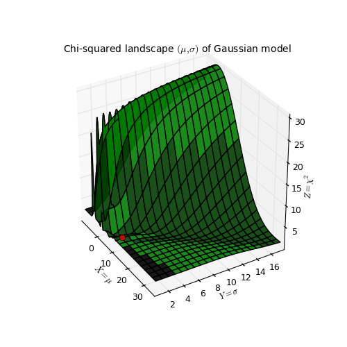
Chi-squared parameter landscape for Gaussian model. The value of chi-squared is plotted along the z-axis.
The figure shows the chi-squared parameter landscape for a model that represents a Gaussian. The landscape axes are model parameters: the position of the peak \(\mu\) and \(\sigma\) which is a measure for the width of the peak (half width at 1/e of peak). The relation between \(\sigma\) and the the full width at half maximum (FWHM) is: \(\mathrm{FWHM} = 2\sigma \sqrt{2ln2} \approx 2.35\, \sigma\). If you imagine this landscape as a solid surface and release a marble, then it rolls to the real minimum (red dot in the figure) only if you are not too far from this minimum. If you start for example in the front right corner, the marble will never end in the real minimum. Note that the parameter space is in fact 4 dimensional (4 free parameters) and therefore more complicated than this example. In the figure we scaled the value for chi-squared to avoid labels with big numbers.
Another representation of the parameter space is a contour plot. It is created by the same example code:
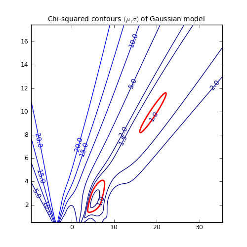
These contour plots are very useful when you compare different objective functions. For instance if you want to compare an objective function for orthogonal fitting with an an objective function for robust fitting.
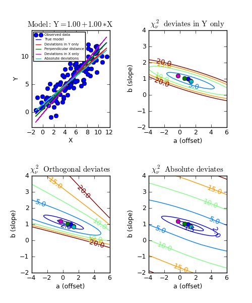
Example: kmpfit_contours_objfunc.py - Comparing objective functions with contour plots
A model which represents a straight line, always shows a very simple landscape with only one minimum. Wherever you release the marble, you will always end up in the real minimum. Then, the quality of the values of the initial estimates are not important to the quality of the fit result.
The initial estimates are entered in parameter params0. You can enter this either in the constructor of the Fitter object or in the method fit(). In most examples we use the latter because then one can repeat the same fit with different initial estimates as in:
fitobj.fit(params0=[1,1])
The results are stored in the attributes of fitobj. For example the best-fit parameters are stored in fitobj.params. For a list of all attributes and their meaning, see the documentation of kmpfit.
An example of an overview of the results could be:
1 2 3 4 5 6 7 8 9 10 11 | print "Fit status: ", fitobj.message
print "Best-fit parameters: ", fitobj.params
print "Covariance errors: ", fitobj.xerror
print "Standard errors ", fitobj.stderr
print "Chi^2 min: ", fitobj.chi2_min
print "Reduced Chi^2: ", fitobj.rchi2_min
print "Iterations: ", fitobj.niter
print "Number of function calls: ", fitobj.nfev
print "Number of free pars.: ", fitobj.nfree
print "Degrees of freedom: ", fitobj.dof
print "Number of pegged pars.: ", fitobj.npegged
|
There is a section about the use and interpretation of parameter errors in Standard errors of best-fit values. In the next chapter we will put the previous information together and compile a complete example.
In this section we explain how to setup a residuals function for kmpfit. We use vectorized functions written with NumPy.
Assume we have data for which we know that the relation between X and Y is a straight line with offset a and slope b, then a model \(f(\mathbf{p},\mathbf{x})\) could be written in Python as:
def model(p, x):
a,b = p
y = a + b*x
return y
Parameter x is a NumPy array and p is a NumPy array containing the model parameters a and b. This function calculates response Y values for a given set of parameters and an array with explanatory X values.
Then it is simple to define the residuals function \(r(\mathbf{p}, [x_i,y_i])\) which calculates the residuals between data points and model:
def residuals(p, data):
x, y = data
return y - model(p,x)
This residuals function has always two parameters. The first one p is an array with parameter values in the order as defined in your model, and data is an object that stores the data arrays that you need in your residuals function. The object could be anything but a list or tuple is often most practical to store the required data. We will explain a bit more about this object when we discuss the constructor of a Fitter object. We need not worry about the sign of the residuals because the fit routine calculates the the square of the residuals itself.
Of course we can combine both functions model and residuals in one function. This is a bit more efficient in Python, but usually it is handy to have the model function available if you need to plot the model using different sets of best-fit parameters.
The objective function which is often used to fit the best-fit parameters of a straight line model is for example:
Assume that the values \(\sigma_i\) are given in array err, then this objective function translates to a residuals function:
def residuals(p, data):
x, y, err = data
ym = a + b*x # Model data
return (y-ym)/err # Squaring is done in Fitter routine
Another example is an objective function for robust (i.e. less sensitive to outliers) for a straight line model without weights. For robust fitting one does not use the square of the residuals but the absolute value.
We cannot avoid that the Fitter routine squares the residuals so to undo this squaring we need to take the square-root as in:
def residuals(p, data):
x, y = data
ym = a + b*x # Model data
r = abs(y - ym) # Absolute residuals for robust fitting
return numpy.sqrt(r) # Squaring is done in Fitter routine
Note
A residuals function should always return a NumPy double-precision floating-point number array (i.e. dtype=’d’).
Note
It is also possible to write residual functions that represent objective functions used in orthogonal fit procedures where both variables x and y have errors. We will give some examples in the section about orthogonal fitting.
For experiments with least square fits, it is often convenient to start with artificial data which resembles the model with certain parameters, and add some Gaussian distributed noise to the y values. This is what we have done in the next couple of lines:
The number of data points and the mean and width of the normal distribution which we use to add some noise:
N = 50
mean = 0.0; sigma = 0.6
Finally we create a range of x values and use our model with arbitrary model parameters to create y values:
xstart = 2.0; xend = 10.0
x = numpy.linspace(3.0, 10.0, N)
paramsreal = [1.0, 1.0]
noise = numpy.random.normal(mean, sigma, N)
y = model(paramsreal, x) + noise
Now we have to tell the constructor of the Fitter object what the residuals function is and which arrays the residuals function needs. To create a Fitter object we use the line:
fitobj = kmpfit.Fitter(residuals=residuals, data=(x,y))
Least squares fitters need initial estimates of the model parameters. As you probably know, our problem is an example of ‘linear regression’ and this category of models have best fit parameters that can be calculated analytically. Then the fit results are not very sensitive to the initial values you supply. So set the values of our initial parameters in the model (a,b) to (0,0). Use these values in the call to Fitter.fit(). The result of the fit is stored in attributes of the Fitter object (fitobj). We show the use of attributes status, message, and params. This last attribute stores the ‘best fit’ parameters, it has the same type as the sequence with the initial parameter (i.e. NumPy array, list or tuple):
paramsinitial = (0.0, 0.0)
fitobj.fit(params0=paramsinitial)
if (fitobj.status <= 0):
print 'Error message = ', fitobj.message
else:
print "Optimal parameters: ", fitobj.params
Below we show a complete example. If you run it, you should get a plot like the one below the source code. It will not be exactly the same because we used a random number generator to add some noise to the data. The plots are created with Matplotlib. A plot is a simple but effective tool to qualify a fit. For most of the examples in this tutorial a plot is included.
Example: kmpfit_example_simple.py - Simple use of kmpfit
1 2 3 4 5 6 7 8 9 10 11 12 13 14 15 16 17 18 19 20 21 22 23 24 25 26 27 28 29 30 31 32 33 34 35 36 37 38 39 40 41 42 43 44 45 46 47 48 49 50 51 52 53 54 55 56 57 58 59 60 61 62 63 64 65 66 67 68 69 70 71 72 73 74 75 76 77 78 79 80 81 82 83 84 | #!/usr/bin/env python
#------------------------------------------------------------
# Purpose: Demonstrate simple use of fitter routine
#
# Vog, 12 Nov 2011
#------------------------------------------------------------
import numpy
from matplotlib.pyplot import figure, show, rc
from kapteyn import kmpfit
# The model
#==========
def model(p, x):
a,b = p
y = a + b*x
return y
# The residual function
#======================
def residuals(p, data):
x, y = data # 'data' is a tuple given by programmer
return y - model(p,x)
# Artificial data
#================
N = 50 # Number of data points
mean = 0.0; sigma = 0.6 # Characteristics of the noise we add
xstart = 2.0; xend = 10.0
x = numpy.linspace(3.0, 10.0, N)
paramsreal = [1.0, 1.0]
noise = numpy.random.normal(mean, sigma, N)
y = model(paramsreal, x) + noise
# Prepare a 'Fitter' object'
#===========================
paramsinitial = (0.0, 0.0)
fitobj = kmpfit.Fitter(residuals=residuals, data=(x,y))
try:
fitobj.fit(params0=paramsinitial)
except Exception, mes:
print "Something wrong with fit: ", mes
raise SystemExit
print "Fit status: ", fitobj.message
print "Best-fit parameters:      ", fitobj.params
print "Covariance errors:        ", fitobj.xerror
print "Standard errors           ", fitobj.stderr
print "Chi^2 min:                ", fitobj.chi2_min
print "Reduced Chi^2:            ", fitobj.rchi2_min
print "Iterations:               ", fitobj.niter
print "Number of function calls: ", fitobj.nfev
print "Number of free pars.:     ", fitobj.nfree
print "Degrees of freedom:       ", fitobj.dof
print "Number of pegged pars.:   ", fitobj.npegged
print "Covariance matrix:\n", fitobj.covar
# Plot the result
#================
rc('font', size=10)
rc('legend', fontsize=8)
fig = figure()
xp = numpy.linspace(xstart-1, xend+1, 200)
frame = fig.add_subplot(1,1,1, aspect=1.0)
frame.plot(x, y, 'ro', label="Data")
frame.plot(xp, model(fitobj.params,xp), 'm', lw=1, label="Fit with kmpfit")
frame.plot(xp, model(paramsreal,xp), 'g', label="The model")
frame.set_xlabel("X")
frame.set_ylabel("Response data")
frame.set_title("Least-squares fit to noisy data using KMPFIT", fontsize=10)
s = "Model: Y = a + b*X real:(a,b)=(%.2g,%.2g), fit:(a,b)=(%.2g,%.2g)"%\
(paramsreal[0],paramsreal[1], fitobj.params[0],fitobj.params[1])
frame.text(0.95, 0.02, s, color='k', fontsize=7,
ha='right', transform=frame.transAxes)
frame.set_xlim(0,12)
frame.set_ylim(0,None)
frame.grid(True)
leg = frame.legend(loc=2)
show()
|
(Source code, png, hires.png, pdf)

For simple fit problems we provide a simple interface. It is a function which is used as follows:
>>> p0 = (0,0)
>>> fitobj = kmpfit.simplefit(model, p0, x, y, err=err, xtol=1e-8)
>>> print fitobj.params
Argument model is a function, just like the model in the previous section. p0 is a sequence with initial values with a length equal to the number of parameters that is defined in your model. Argument x and y are the arrays or lists that represent your measurement data. Argument err is an array with 1 \(\sigma\) errors, one for each data point. Then you can enter values to tune the fit routine with keyword arguments (e.g. gtol, xtol, etc.). In the next example we demonstrate how to use lists for your data points, how to make an unweighted fit and how to print the right parameter uncertainties. For an explanation of parameter uncertainties, see section Standard errors of best-fit values.
The advantages of this function:
- You need only to worry about a model function
- No need to create a Fitter object first
- Direct input of relevant arrays
- As a result you get a Fitter object with all the attributes
- It is (still) possible to tune the fit routine with keyword arguments, no limitations here.
Example: kmpfit_example_easyinterface.py - Simple function
1 2 3 4 5 6 7 8 9 10 11 12 13 14 15 16 17 18 19 20 21 22 23 24 25 26 27 28 29 30 31 32 33 34 35 36 37 38 39 40 41 42 | #!/usr/bin/env python
#------------------------------------------------------------
# Purpose: Demonstrate simple use of fitter routine
#
# Vog, 24 Nov 2011
#------------------------------------------------------------
import numpy
from matplotlib.pyplot import figure, show
from kapteyn import kmpfit
# The model:
def model(p, x):
a, b = p
y = a + b*x
return y
# Artificial data
N = 50 # Number of data points
mean = 0.0; sigma = 0.6 # Characteristics of the noise we add
x = numpy.linspace(2, 10, N)
paramsreal = [1.0, 1.0]
noise = numpy.random.normal(mean, sigma, N)
y = model(paramsreal, x) + noise
err = numpy.random.normal(mean, sigma, N)
# Simple interface
p0 = (0,0)
xl = range(10)
yl = [k*0.5 for k in xl]
fitobj = kmpfit.simplefit(model, p0, xl, yl)
print "Best fit parameters:", fitobj.params
print "Parameter errors: :", fitobj.stderr
fitobj = kmpfit.simplefit(model, p0, x, y, err=err, xtol=1e-8)
print "Best fit parameters:", fitobj.params
print "Parameter errors: :", fitobj.xerror
fitobj = kmpfit.simplefit(model, p0, x, y, maxiter=100)
print "Best fit parameters:", fitobj.params
print "Parameter errors: :", fitobj.stderr
|
With the estimation of errors on the best-fit parameters we get an idea how good a fit is. Usually these errors are called standard errors, but often programs call these errors also standard deviations. For nonlinear least-squares routines, these errors are based on mathematical simplifications and are therefore often called asymptotic or approximate standard errors.
The standard error (often denoted by SE) is a measure of the average amount that the model over- or under-predicts.
According to [Bev] , the standard error is an uncertainty which corresponds to an increase of \(\chi^2\) by 1. That implies that if we we add the standard error \(\sigma_i\) to its corresponding parameter, fix it in a second fit and fit again, the value of \(\chi^2\) will be increased by 1.
The next example shows this behaviour. We tested it with the first parameter fixed and a second time with the second parameter fixed. The example also shows how to set parameters to ‘fixed’ in kmpfit. The model is a straight line. If you run the example you will see that it shows exactly the behaviour as in (7). This proves that the covariance matrix (explained later) of kmpfit can be used to derive standard errors. Note the use of the parinfo attribute of the Fitter object to fix parameters. One can use an index to set values for one parameter or one can set the values for all parameters. These values are given as a Python dictionary. An easy way to create a dictionary is to use Python’s dict() function.
Example: kmpfit_errors_chi2delta.py - Meaning of asymptotic errors
1 2 3 4 5 6 7 8 9 10 11 12 13 14 15 16 17 18 19 20 21 22 23 24 25 26 27 28 29 30 31 32 33 34 35 36 37 38 39 40 41 42 43 44 45 46 47 48 49 50 51 52 53 54 55 56 57 58 59 60 61 62 63 | #!/usr/bin/env python
#------------------------------------------------------------
# Purpose: Demonstrate, using kmpfit, that if you find best-fit
# parameters, the errors derived from the covariance matrix
# correspond to an increase in chi^2 of 1.
# Vog, 23 Nov 2011
#------------------------------------------------------------
import numpy
from matplotlib.pyplot import figure, show, rc
from numpy.random import normal, randint
from kapteyn import kmpfit
def residuals(p, data):
x, y, err = data
a, b = p
model = a + b*x
return (y-model)/err
# Artificial data
#----------------
N = 100
a0 = 2; b0 = 3
x = numpy.linspace(0.0, 2.0, N)
y = a0 + b0*x + normal(0.0, 0.4, N) # Mean,sigma,N
derr = normal(0.0, 0.5, N)
err = 0.9+derr
fitobj = kmpfit.Fitter(residuals=residuals, data=(x, y, err))
fitobj.fit(params0=[1,1])
if (fitobj.status <= 0):
print 'error message =', fitobj.errmsg
raise SystemExit
print "\n\n======== Results kmpfit for Y = A + B*X ========="
print "Params: ", fitobj.params
print "Errors from covariance matrix : ", fitobj.xerror
print "Uncertainties assuming reduced Chi^2=1: ", fitobj.stderr
print "Chi^2 min: ", fitobj.chi2_min
p1, p2 = fitobj.params
e1, e2 = fitobj.xerror
# Next we take one of the parameters to be fixed and change its value
# with the amount of one of the estimated errors (covariance, scaled or bootstrap)
# If we fit again, then, according to Bevington (Data Reduction and Error
# Analysis for the Physical Sciences Section 11-5), one should expect the
# Chi square value to increase with 1.0
fitobj.parinfo[0] = dict(fixed=True)
fitobj.fit(params0=[p1+e1,1])
print "\nFix first parameter and set its value to fitted value+error"
print "Params: ", fitobj.params
print "Chi^2 min: ", fitobj.chi2_min
print "Errors from covariance matrix : ", fitobj.xerror
fitobj.parinfo = [{'fixed':False}, {'fixed':True}]
fitobj.fit(params0=[1, p2+e2])
print "\nFix second parameter and set its value to fitted value+error"
print "Params: ", fitobj.params
print "Chi^2 min: ", fitobj.chi2_min
print "Errors from covariance matrix : ", fitobj.xerror
|
The results for an arbitrary run:
1 2 3 4 5 6 7 8 9 10 11 12 13 14 15 | ======== Results kmpfit for Y = A + B*X =========
Params: [2.0104270702631712, 2.94745915643011]
Errors from covariance matrix : [ 0.05779471 0.06337059]
Uncertainties assuming reduced Chi^2=1: [ 0.04398439 0.04822789]
Chi^2 min: 56.7606029739
Fix first parameter and set its value to fitted value+error
Params: [2.0682217814912143, 2.896736695408106]
Chi^2 min: 57.7606030002
Errors from covariance matrix : [ 0. 0.03798767]
Fix second parameter and set its value to fitted value+error
Params: [1.9641675954511788, 3.0108297500339498]
Chi^2 min: 57.760602835
Errors from covariance matrix : [ 0.0346452 0. ]
|
As you can see, the value of chi-square has increased with ~1.
In the literature [Num] we can find analytical expressions for the standard errors of weighted fits for standard linear regression. We want to discuss the derivation of analytical errors for weighted fits to demonstrate that these errors are also represented by the elements of the so-called variance-covariance matrix (or just covariance matrix), which is also a result of a fit with kmpfit (attribute Fitter.covar). How should we interpret these errors? For instance in Numerical Recipes, [Num] we find the expressions for the best fit parameters of a model \(y=a+bx\) Use the chi-squared objective function:
To find analytical expressions for the best-fit values of a and b, we need to take derivatives of this objective function:
Define:
Then one can rewrite (9) into:
which is in matrix notation:
If we define:
which gives the solution:
Define:
The solutions for a and b are:
For the standard errors we will derive the error in parameter a and b. The error in a is by the law of propagation of errors:
>From (16) and (10) we derive:
With (17) we find
Applying the same procedure to b:
With (17) we find
To summarize:
A classical implementation to find analytical best-fit parameters using NumPy is as follows:
1 2 3 4 5 6 7 8 9 10 11 12 13 14 | def lingres(xa, ya, err):
w = numpy.where(err==0.0, 0.0, 1.0/(err*err))
Sum = w.sum()
sumX = (w*xa).sum()
sumY = (w*ya).sum()
sumX2 = (w*xa*xa).sum()
sumY2 = (w*ya*ya).sum()
sumXY = (w*xa*ya).sum()
delta = Sum * sumX2 - sumX * sumX
a = (sumX2*sumY - sumX*sumXY) / delta
b = (sumXY*Sum - sumX*sumY) / delta
siga = numpy.sqrt(abs(sumX2/delta))
sigb = numpy.sqrt(abs(Sum/delta))
return a, b, siga, sigb, delta, Sum, sumX2, sumX
|
Note that these formulas are susceptible to roundoff error and Numerical Recipes derives alternative formulas (Section 15.2). However, our functions work with double precision numbers and we didn’t (yet) encounter a situation where roundoff errors were obvious.
If we compare these results with the elements of the covariance matrix in (13), then we observe that the expressions for the parameter variances, are the square root of the diagonal values of this matrix. The co-variance between a and b can be calculated also and the formula turns out to be the same as the off-diagonal elements of the covariance matrix. This value is:
It is easy to demonstrate that these errors are the same as those we find with kmpfit in attribute xerror, which are the square-root diagonal values of the covariance matrix in attribute covar.
The covariance matrix elements \(C_{jk}\) for best-fit parameters p can be written as:
where we used j to indicate the matrix row and k the matrix column. If j=k then:
from which follows that the square root of the diagonal elements of the covariance matrix are the estimates of the best-fit parameter uncertainties.
Note
Example program kmpfit_linearreg.py compares the analytical covariance matrix with the kmpfit version for linear regression, using the previously derived formulas in this section. The output of an arbitrary example run demonstrates the similarity between the analytical and the kmpfit method:
Example: kmpfit_linearreg.py - Compare output analytical method and kmpfit
1 2 3 4 5 6 7 8 9 10 11 12 13 14 15 16 17 | -- Results analytical solution:
Best fit parameters: [0.57857142857143595, 5.5285714285714258]
Parameter errors weighted fit: [0.84515425472851657, 0.1889822365046136]
Parameter errors un-/relative weighted fit: [1.0696652156022404, 0.2391844135253578]
Minimum chi^2: 8.00928571429
Covariance matrix:
0.714285714286 -0.142857142857
-0.142857142857 0.0357142857143
-- Results kmpfit:
Best-fit parameters: [0.57857145533008425, 5.5285714226701863]
Parameter errors weighted fit: [ 0.84515434 0.18898225]
Parameter errors un-/relative weighted fit: [ 1.06966532 0.23918443]
Minimum chi^2: 8.00928571429
Covariance matrix:
[[ 0.71428585 -0.14285717]
[-0.14285717 0.03571429]]
|
We observe:
- The analytical values of the best-fit parameters and those from kmpfit correspond. The same applies to the errors for the unweighted fit/fit with relative weights.
Sometimes there is a good reason to use a fit method that can deal with weights. Usually you assign weights if you have additional knowledge about your measurements. Some points get more weight if they are more reliable than others. Therefore you should expect that the best-fit parameters are different between weighted and un-weighted fits. Also the accuracy of the results will improve, because besides the data you are using the quality of the data. The difference in best-fit parameters and the quality of the results is shown with program kmpfit_compare_wei_unwei.py
Example: kmpfit_compare_wei_unwei.py - Compare output for unweighted (unit weighting) and weighted fit
1 2 3 4 5 6 7 8 9 10 11 12 13 14 15 16 17 18 19 | Data x: [ 1. 2. 3. 4. 5. 6. 7.]
Data y: [ 6.9 11.95 16.8 22.5 26.2 33.5 41. ]
Errors: [ 0.05 0.1 0.2 0.5 0.8 1.5 4. ]
-- Results kmpfit unit weighting wi=1.0:
Best-fit parameters: [0.57857145533008425, 5.5285714226701863]
Parameter errors weighted fit: [ 0.84515434 0.18898225]
Minimum chi^2: 8.00928571429
Covariance matrix:
[[ 0.71428585 -0.14285717]
[-0.14285717 0.03571429]]
-- Results kmpfit with weights:
Best-fit parameters: [1.8705399823164173, 5.0290902421858439]
Parameter errors weighted fit: [ 0.09922304 0.06751229]
Minimum chi^2: 4.66545480308
Covariance matrix:
[[ 0.00984521 -0.00602421]
[-0.00602421 0.00455791]]
|
If you examine the residuals function in this program, you will observe that we use a weight of \(1/err_i\) in the residuals function, which is squared by kmpfit, so in fact the weighting is \(1/\sigma_i^2\). First we set all the errors to 1.0. This is called unit weighting and effectively this fit does not weight at all. The second fit has different weights. Important is the observation that these weights can be relative. Then they contain information about the quality of the data but do not necessarily contain correct information about the errors on the data points and therefore give incorrect errors on the parameter estimates. This is shown in the same program kmpfit_compare_wei_unwei.py where we scaled the errors with a factor 10. The errors in the parameter estimates are increased by a factor 10.
Example: kmpfit_compare_wei_unwei.py - Compare output for unweighted (unit weighting) and weighted fit
-- Results kmpfit with scaled individual errors (factor=10):
Best-fit parameters: [1.870539984453957, 5.0290902408769238]
Parameter errors weighted fit: [ 0.99223048 0.6751229 ]
Minimum chi^2: 0.0466545480308
Covariance matrix:
[[ 0.98452132 -0.60242076]
[-0.60242076 0.45579092]]
This demonstrates that if weights are relative or when unit weighting is applied, one cannot rely on the covariance errors to represent real errors on the parameter estimates. The covariance errors are still based on a change in \(\chi^2\) of 1.0, but the weights do not represent the variances of the data correctly.
To summarize the weighting schemes:
- Unweighted or unit weighting. Set \(w_i=1/\sigma_i^2\) to 1.0
- Relative weighting. Set \(w_i=1/\sigma_i^2\) but the errors on the parameter estimates in kmpfit‘s attribute xerror cannot be used.
- Statistical weighting. Set \(w_i=1/\sigma_i^2\). The errors on the parameter estimates in kmpfit‘s attribute xerror are correct. An important assumption of this method is that the error distribution of the measured data is Gaussian and that the data errors are measured accurately (absolute uncertainties).
- Other weighting schemes like Poisson weighting \(w_i=1/y_i\)
>From the theory of maximum likelihood we find that for a least squares solution we need to maximize the probability that a measurement \(y_i\) with given \(\sigma_i\) is in a a small interval \(dy_i\) around \(y_i\) by minimizing the sum chi squared [Ds1] :
with:
- N is the number of data points
- \(y_i\) the measured data at \(x_i\)
- \(\sigma_i\) is the standard deviation of measurement i
- f is the model for which we want to find the best-fit parameters.
The sum is often called chi squared because it follows the \(\chi^2\) distribution if we repeat the experiment to get new measurements. The expectation value of \(\chi^2\) is (see proof in [Ds3]):
where n is the number of free parameters in the fit. The reduced chi squared \(\chi_{\nu}^2\) is defined as:
where \(\nu = N-n\). From (27) we derive for the expectation value of \(\chi_{\nu}^2\):
Fitting with (26) as objective function is often called chi squared fitting. The value of \(\chi^2_{\nu}\) is a measure of the goodness of fit and is returned by kmpfit in a Fitter object as attribute rchi2_min. The number of degrees of freedom is stored in attribute dof.
Note
In the literature we find relations between the standard deviation of the sample and the true standard deviation of the underlying distribution . For least squares analysis we replace the average value of y (i.e. \(\bar{y}\)) in those formulas by the model with the best-fit parameters \(f(p,x)\).
What should we expect of the variance \(\sigma_i\) compared to the sample deviations for each sample point? Assume we have N data points and each data point has an individual error of \(\sigma_i\). >From (27) we have:
With the observation that the expectation value of each of the N terms is the same we derive for each data point:
So for a good fit the true deviation of a measurement \(\sigma_i\) for large N is almost equal to the deviation between data point and fit. The less the scatter of data about the best fit, the smaller \(\sigma_i\) should be.
The sample variance, \(s_y^2\) is then written as [Ds2] :
If we replace all \(\sigma_i\) with \(\sigma_y\) in equation (30), then we derive a familiar relationship:
so that the value of \(s_y^2\) of the measurements is an unbiased estimate of the true variance \(\sigma_y^2\) of the underlying distribution. For an unbiased estimator, the expected value and the true value are the same.
The weighted version of the sample variance is defined as:
If we use \(1/\sigma_i^2\) as weight, then:
Bevington [Bev] defines the weighted average of the individual variances \(\bar{\sigma}_i^2\) as:
Then:
If we set all weights to the same value \(w_i=1/\sigma_y^2\) then \(sw_y = s_y\) and:
which is consistent with (33).
For chi squared fitting it is therefore important to have correct values for \(\sigma_i\). Over-estimated values give a \(\chi^2_{\nu}\) which is smaller than 1 and under-estimated values give a value bigger than 1 (If you get very large values, then probably fit and data are not in agreement). If the values for \(\sigma_i\) are unreliable then also the error estimates of the best-fit parameters are unreliable, because they are functions of \(\sigma_i\) (see e.g. the analytical expressions for these errors in a linear regression in (22)). According to equations (37) and (38) it is reasonable then to scale the values of \(\sigma_i\) in a way that we force \(\chi^2_{\nu}\) to take its expectation value of 1. Then one gets values for the errors in stderr which are insensitive to arbitrary scaling factors of the weights.
We noted earlier that scaling the weights does not change the values of the best-fit parameters but they affect the values of the parameter error estimates because they depend on the values of \(\sigma_i\). If for example values of \(\sigma_i\) are all too small with a factor 2 with respect to those that make \(\chi_{\nu} =1\). Then the errors in the parameter estimates are to small with a factor 2x2=4 (see e.g. (19) and (21) for the straight line model). The value of \(\chi_{\nu}\) will be 2x2=4. So to correct the errors on the parameter estimates, we can multiply the variances with the value of \(\chi_{\nu}\). If we recall equation (25), then we see that this scaling can be applied to arbitrary models. This scaling is exactly what happens in kmpfit for the values in attribute stderr.
In kmpfit we use the unit- or relative weights as given by the user and calculate the value of \(\chi_{\nu}\). The asymptotic standard errors in xerror are then multiplied by the square root of the value of \(\chi_{\nu}\) and stored in attribute stderr. We demonstrate this with the output of a small example (kmpfit_compare_wei_unwei.py) with data from [Wol]:
Example: kmpfit_compare_wei_unwei.py - Compare output for unweighted (unit weighting) and weighted fit
1 2 3 4 5 6 7 8 9 10 11 12 13 14 15 16 17 18 | Data x: [ 1. 2. 3. 4. 5. 6. 7.]
Data y: [ 6.9 11.95 16.8 22.5 26.2 33.5 41. ]
Errors: [ 0.05 0.1 0.2 0.5 0.8 1.5 4. ]
New array with measurement errors, scaled with factor 0.933091 to give
a reduced chi-squared of 1.0:
[ 0.04829832 0.09659663 0.19319327 0.48298317 0.77277307 1.4489495
3.86386534]
-- Results kmpfit with scaled individual errors to force red_chi2=1:
Best-fit parameters: [1.8705399822570359, 5.029090242191204]
Parameter errors using measurement uncertainties: [ 0.09584612 0.0652146 ]
Parameter errors unit-/relative weighted fit: [ 0.09584612 0.0652146 ]
Minimum chi^2: 5.0
Minimum reduced chi^2: 1.0
Covariance matrix:
[[ 0.00918648 -0.00562113]
[-0.00562113 0.00425294]]
|
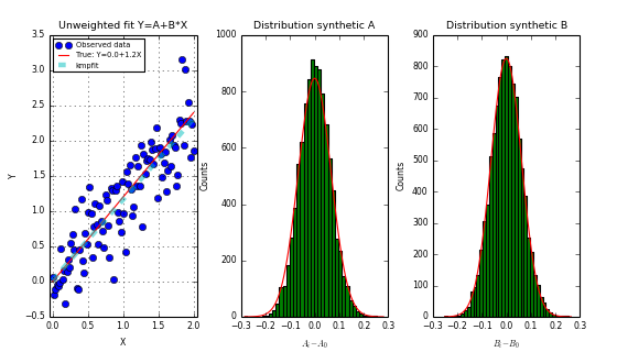
The next code example is a small script that shows that the scaled error estimates in attribute stderr for unit- and relative weighting are realistic if we compare them to errors found with a Monte Carlo method. We start with values of \(\sigma_i\) that are under-estimated. This results in a value for \(\chi_{\nu}\) which is too low. The re-scaled errors in stderr match with those that are estimated with the Monte-Carlo method. In the example we used the Bootstrap Method. The plot shows the fit and the bootstrap distributions of parameter A and B. We will explain the Bootstrap Method in the next section.
Example: kmpfit_unweighted_bootstrap_plot.py - How to deal with unweighted fits
1 2 3 4 5 6 7 8 9 10 11 12 13 14 15 16 17 18 19 20 21 22 23 24 25 26 27 28 29 30 31 32 33 34 35 36 37 38 39 40 41 42 43 44 45 46 47 48 49 50 51 52 53 54 55 56 57 58 59 60 61 62 63 64 65 66 67 68 69 70 71 72 73 74 75 76 77 78 79 80 81 82 83 84 85 86 87 88 89 90 91 92 93 94 95 96 97 98 99 100 101 102 103 104 105 106 107 108 109 110 111 112 113 114 115 116 117 | #!/usr/bin/env python
#------------------------------------------------------------
# Purpose: Demonstrate that the scaled covariance errors for
# unweighted fits are comparable to errors we find with
# a bootstrap method.
# Vog, 24 Nov 2011
#------------------------------------------------------------
import numpy
from matplotlib.pyplot import figure, show, rc
from numpy.random import normal, randint
from kapteyn import kmpfit
# Residual and model in 1 function. Model is straight line
def residuals(p, data):
x, y, err = data
a, b = p
model = a + b*x
return (y-model)/err
# Artificial data
N = 100
a0 = 0; b0 = 1.2
x = numpy.linspace(0.0, 2.0, N)
y = a0 + b0*x + normal(0.0, 0.4, N) # Mean,sigma,N
err = numpy.ones(N) # All weights equal to 1
# Prepare fit routine
fitobj = kmpfit.Fitter(residuals=residuals, data=(x, y, err))
try:
fitobj.fit(params0=[1,1])
except Exception, mes:
print "Something wrong with fit: ", mes
raise SystemExit
print "\n\n======== Results kmpfit unweighted fit ========="
print "Params: ", fitobj.params
print "Errors from covariance matrix : ", fitobj.xerror
print "Uncertainties assuming reduced Chi^2=1: ", fitobj.stderr
print "Chi^2 min: ", fitobj.chi2_min
print "Reduced Chi^2: ", fitobj.rchi2_min
print "Iterations: ", fitobj.niter
print "Function ev: ", fitobj.nfev
print "Status: ", fitobj.status
print "Status Message:", fitobj.message
# Bootstrap method to find uncertainties
A0, B0 = fitobj.params
xr = x.copy()
yr = y.copy()
ery = err.copy()
fitobj = kmpfit.Fitter(residuals=residuals, data=(xr, yr, ery))
slopes = []
offsets = []
trials = 10000 # Number of synthetic data sets
for i in range(trials): # Start loop over pseudo sample
indx = randint(0, N, N) # Do the resampling using an RNG
xr[:] = x[indx]
yr[:] = y[indx]
ery[:] = err[indx]
# Only do a regression if there are at least two different
# data points in the pseudo sample
ok = (xr != xr[0]).any()
if (not ok):
print "All elements are the same. Invalid sample."
print xr, yr
else:
fitobj.fit(params0=[1,1])
offs, slope = fitobj.params
slopes.append(slope)
offsets.append(offs)
slopes = numpy.array(slopes) - B0
offsets = numpy.array(offsets) - A0
sigmaA0, sigmaB0 = offsets.std(), slopes.std()
print "Bootstrap errors in A, B:", sigmaA0, sigmaB0
# Plot results
rc('font', size=7)
rc('legend', fontsize=6)
fig = figure(figsize=(7,4))
fig.subplots_adjust(left=0.08, wspace=0.3, right=0.94)
frame = fig.add_subplot(1,3,1, aspect=1.0, adjustable='datalim')
frame.plot(x, y, 'bo', label='Observed data')
frame.plot(x, a0+b0*x, 'r', label='True: Y=%.1f+%.1fX'%(a0,b0))
frame.plot(x, A0+B0*x, '--c', alpha=0.5, lw=4, label='kmpfit')
frame.set_xlabel("X"); frame.set_ylabel("Y")
frame.set_title("Unweighted fit Y=A+B*X")
frame.grid(True)
frame.legend(loc='upper left')
ranges = [(offsets.min(), offsets.max()),(slopes.min(), slopes.max())]
nb = 40 # Number of bins in histogram
for i,sigma in enumerate([sigmaA0, sigmaB0]):
framehist = fig.add_subplot(1, 3, 2+i)
range = ranges[i] # (X) Range in histogram
framehist.hist(slopes, bins=nb, range=range, fc='g')
binwidth = (range[1]-range[0])/nb # Get width of one bin
area = trials * binwidth # trials is total number of counts
mu = 0.0
amplitude = area / (numpy.sqrt(2.0*numpy.pi)*sigma)
x = numpy.linspace(range[0], range[1], 100)
y = amplitude * numpy.exp(-(x-mu)*(x-mu)/(2.0*sigma*sigma))
framehist.plot(x, y, 'r')
if i == 0:
lab = "$A_i-A_0$"
title = "Distribution synthetic A"
else:
lab = "$B_i-B_0$"
title = "Distribution synthetic B"
framehist.set_xlabel(lab)
framehist.set_ylabel("Counts")
framehist.set_title(title)
show()
|
(Source code, png, hires.png, pdf)
We need to discuss the bootstrap method, that we used in the last script, in some detail. Bootstrap is a tool which estimates standard errors of parameter estimates by generating synthetic data sets with samples drawn with replacement from the measured data and repeating the fit process with this synthetic data.
Your data realizes a set of best-fit parameters, say \(p_{(0)}\). This data set is one of many different data sets that represent the ‘true’ parameter set \(p_{true}\) . Each data set will give a different set of fitted parameters \(p_{(i)}\). These parameter sets follow some probability distribution in the n dimensional space of all possible parameter sets. To find the uncertainties in the fitted parameters we need to know the distribution of \(p_{(i)}-p_{true}\) [Num]. In Monte Carlo simulations of synthetic data sets we assume that the shape of the distribution of Monte Carlo set \(p_{(i)}-p_{0}\) is equal to the shape of the real world set \(p_{(i)}-p_{true}\)
The Bootstrap Method [Num] uses the data set that you used to find the best-fit parameters. We generate different synthetic data sets, all with N data points, by randomly drawing N data points, with replacement from the original data. In Python we realize this as follows:
indx = randint(0, N, N) # Do the re-sampling using an RNG
xr[:] = x[indx]
yr[:] = y[indx]
ery[:] = err[indx]
We create an array with randomly selected array indices in the range 0 to N. This index array is used to create new arrays which represent our synthetic data. Note that for the copy we used the syntax xr[:] with the colon, because we want to be sure that we are using the same array xr, yr and ery each time, because the fit routine expects the data in these arrays (and not copies of them with the same name). The synthetic data arrays will consist of about 37 percent duplicates. With these synthetic arrays we repeat the fit and find our \(p_{(i)}\). If we repeat this many times (let’s say 1000), then we get the distribution we needed. The standard deviation of this distribution (i.e. for one parameter), gives the uncertainty.
Note
The bigger the data set, the higher the number of bootstrap trials should be to get accurate statistics. The best way to find a minimum number is to plot the Bootstrap results as in the example.
Another Monte Carlo method is the Jackknife method. The Jackknife method finds errors on best-fit parameters of a model and N data points using N samples. In each sample a data point is left out, starting with the first, then the second and so on. For each of these samples we do a fit and store the parameters. For example, for a straight line we store the slopes and offsets. If we concentrate on one parameter and call this parameter \(\theta\) then for each run i we find the estimated slope \(\theta_i\). The average of all the slopes is \(\bar{\theta^*})\). Then the Jackknife error is:
Unweighted (i.e. unit weighting) and relative weighted fits
- For unit- or relative weighting, we find errors that correspond to attribute stderr in kmpfit.
- The errors on the best-fit parameters are scaled (internally) which is equivalent to scaling the weights in a way that the value of the reduced chi-squared becomes 1.0
- For unweighted fits, the standard errors from Fitter.stderr are comparable to errors we find with Monte Carlo simulations.
Alper, [Alp] states that for some combinations of model, data and weights, the standard error estimates from diagonal elements of the covariance matrix neglect the interdependencies between parameters and lead to erroneous results. Often the measurement errors are difficult to obtain precisely, sometimes these errors are not normally distributed. For this category of weighting schemes, one should always inspect the covariance matrix (attribute covar) to get an idea how big the covariances are with respect to the variances (diagonal elements of the matrix). The off-diagonal elements of the covariance matrix should be much lower than the diagonal.
Weighted fits with weights derived from real measurement errors
- For weighted fits where the weigths are derived from measurement errors, the errors correspond to attribute xerror in kmpfit. Only for this type of weights, we get a value of (reduced) chi-squared that can be used as a measure of goodness of fit.
- The fit results depend on the accuracy of the measurement errors \(\sigma_i.\)
- A basic assumption of the chi-squared objective function is that the error distribution of the measured data is Gaussian. If this assumption is violated, the value of chi squared does not make sense.
- The uncertainties given in attribute xerror and stderr are the same, only when \(\chi_{\nu}^2 = 1\)
>From [And] we summarize the conditions which must be met before one can safely use the values in stderr (i.e. demanding that \(\chi_{\nu} = 1\)): In this approach of scaling the error in the best-fit parameters, we make some assumptions:
- The error distribution has to be Gaussian.
- The model has to be linear in all parameters. If the model is nonlinear, we cannot demand that \(\chi_{\nu} = 1\), because the derivation of \(\langle\chi\rangle^2=N-n\) implicitly assumes linearity in all parameters.
- By demanding \(\chi_{\nu} = 1\), we explicitly claim that the model we are using is the correct model that corresponds to the data. This is a rather optimistic claim. This claim requires justification.
- Even if all these assumptions above are met, the method is in fact only applicable if the degrees of freedom N-n is large. The reason is that the uncertainty in the measured data data does not only cause an uncertainty in the model parameters, but also an uncertainty in the value of \(\chi^2\) itself. If N-n is small, \(\chi^2\) may deviate substantially from N-n even though the model is linear and correct.
The conclusion is that one should be careful with the use of standard errors in stderr. A Monte Carlo method should be applied to prove that the values in stderr can be used. For weighted fits it is advertised not to use the Bootstrap method. In the next example we compare the Bootstrap method with and without weights. The example plots all trial results in the Bootstrap procedure. The yellow lines represent weighted fits in the Bootstrap procedure. The green lines represent unweighted fits in the Bootstrap procedure. One can observe that the weighted version shows errors that are much too big.
Example: kmpfit_weighted_bootstrap.py - Compare Bootstrap with weighted and unweighted fits
1 2 3 4 5 6 7 8 9 10 11 12 13 14 15 16 17 18 19 20 21 22 23 24 25 26 27 28 29 30 31 32 33 34 35 | ======== Results kmpfit UNweighted fit =========
Params: [-0.081129823700123893, 2.9964571786959704]
Errors from covariance matrix : [ 0.12223491 0.0044314 ]
Uncertainties assuming reduced Chi^2=1: [ 0.21734532 0.00787946]
Chi^2 min: 626.001387167
Reduced Chi^2: 3.16162316751
Iterations: 2
Function ev: 7
Status: 1
======== Results kmpfit weighted fit =========
Params: [-1.3930156818836363, 3.0345053718712571]
Errors from covariance matrix : [ 0.01331314 0.0006909 ]
Uncertainties assuming reduced Chi^2=1: [ 0.10780843 0.00559485]
Chi^2 min: 12984.0423449
Reduced Chi^2: 65.575971439
Iterations: 3
Function ev: 7
Status: 1
Covariance matrix: [[ 1.77239564e-04 -6.78626129e-06]
[ -6.78626129e-06 4.77344773e-07]]
===== Results kmpfit weighted fit with reduced chi^2 forced to 1.0 =====
Params: [-1.3930155828717012, 3.034505368057717]
Errors from covariance matrix : [ 0.10780841 0.00559485]
Uncertainties assuming reduced Chi^2=1: [ 0.10780841 0.00559485]
Chi^2 min: 198.0
Reduced Chi^2: 1.0
Iterations: 3
Function ev: 7
Status: 1
Bootstrap errors in A, B for procedure with weighted fits: 0.949585141866 0.0273199443168
Bootstrap errors in A, B for procedure with unweighted fits: 0.217752459166 0.00778497229684
|
(Source code, png, hires.png, pdf)

The same conclusion applies to the Jackknife method. For unweighted fits, the Jackknife error estimates are very good, but for weighted fits, the method can not be used. This can be verified with the example script below. [Sha] proposes a modified Jackknife method to improve the error estimates.
Example: kmpfit_weighted_jackknife.py - Compare Jackknife with weighted and unweighted fits
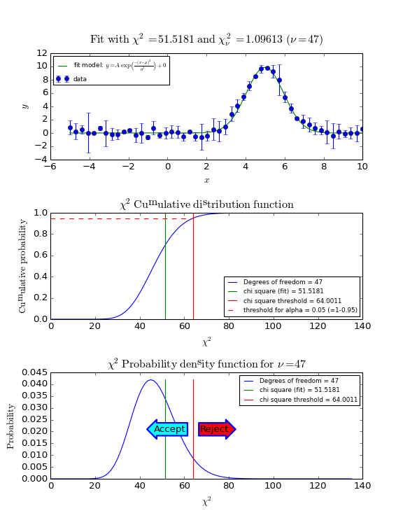
As described in a previous section, the value of the reduced chi-squared is an indication for the goodness of fit. If its value is near 1 then your fit is probably good. With the value of chi-squared we can find a threshold value for which we can accept or reject the hypothesis that the data and the fitted model are consistent. The assumption is that the value of chi-squared follows the \(\chi^2\) distribution with \(\nu\) degrees of freedom. Let’s examine chi-squared in more detail.
In a chi-squared fit we sum the relative size of the deviation \(\Delta_i\) and the error bar \(\delta_i\). Data points that are near the fit with the best-fit parameters have a small value \(\Delta_i/\delta_i\). Bad points have a ratio that is bigger than 1. At those points the fitted curve does not go through the error bar. For a reasonable fit, there will be both small and big deviations but on average the value will be near 1. Remember that chi-squared is defined as:
So if we expect that on average the ratios are 1, then we expect that this sum is equal to N. You can always add more parameters to a model. If you have as many parameters as data points, you can find a curve that hits all data points, but usually these curves have no significance. In this case you don’t have any degrees of freedom. The degrees of freedom for a fit with N data points and n adjustable model parameters is:
To include the degrees of freedom, we define the reduced chi squared as:
In the literature ([Ds3]) we can find prove that the expectation value of the reduced chi squared is 1. If we repeat a measurement many times, then the measured values of \(\chi^2\) are distributed according to the chi-squared distribution with \(\nu\) degrees of freedom. See for example http://en.wikipedia.org/wiki/Chi-squared_distribution.
We reject the null hypothesis (data is consistent with the model with the best fit parameters) if the value of chi-squared is bigger than some threshold value. The threshold value can be calculated if we set a value of the probability that we make a wrong decision in rejecting a true null hypothesis (H0). This probability is denoted by \(\alpha\) and it sets the significance level of the test. Usually we want small values for \(\alpha\) like 0.05 or 0.01. For a given value of \(\alpha\) we calculate \(1-\alpha\), which is the left tail area under the cumulative distribution function. This probability is calculated with scipy.stats.chi2.cdf(). If \(\alpha\) is given and we want to know the threshold value for chi-squared, then we use the Percent Point Function scipy.stats.chi2.ppf() which has \(1-\alpha\) as its argument.
The recipe to obtain a threshold value for \(\chi^2\) is as follows.
- Set the hypotheses:
- \(H_0\): The data are consistent with the model with the best fit parameters
- \(H_{\alpha}\): The data are not consistent with the model with the best fit parameters
Make a fit and store the calculated value of \(\chi^2\)
Set a p-value (\(\alpha\))
Use the \(\chi^2\) cumulative distribution function for \(\nu\) degrees of freedom to find the threshold \(\chi^2\) for \(1-\alpha\). Note that \(\alpha\) is the right tailed area in this distribution while we use the left tailed area in our calculations.
Compare the calculated \(\chi^2\) with the threshold value.
If the calculated value is bigger, then reject the hypothesis that the data and the model with the best-fit parameters are consistent.
In the next figure we show these steps graphically. Note the use of the statistical functions and methods from SciPy.
Example: kmpfit_goodnessoffit1.py - Goodness of fit based on the value of chi-squared
(Source code, png, hires.png, pdf)
Another goodness-of-fit test is constructed by using the critical values of the Kolmogorov distribution (Kolmogorov-Smirnov test [Mas] ).
For this test we need the normalized cumulative versions of the data and the model with the best-fit parameters. We call the cumulative distribution function of the model \(F_0(x)\) and the observed cumulative distribution function of our data sample \(S_n(x)\) then the sampling distribution of \(D = \max| F_0(x) - S_n(x) |\) follows the Kolmogorov distribution which is independent of \(F_0(x)\) if \(F_0(x)\) is continuous, i.e. has no jumps.
The cumulative distribution of the sample is called the empirical distribution function (ECDF). To create the ECDF we need to order the sample values \(y_0, y_1, ..., y_n\) from small to high values. Then the ECDF is defined as:
The value of \(n(i)\) is the number of sample values \(y\) that are smaller than or equal to \(y_i\). So the first value would be 1/N, the second 2/N etc.
The cumulative distribution function (CDF) of the model can be calculated in the same way. First we find the best-fit parameters for a model using kmpfit. Select a number of X values to find Y values of your model. Usually the number of model samples is much higher than the number of data samples. With these (model) Y values we create a CDF using the criteria (ordered Y values) of the data. If dat1 are the ordered sample Y values and dat2 are the ordered model Y values, then a function that calculates the CDF could be:
def cdf(Y_ord_data, Y_ord_model):
cdfnew = []
n = len(Y_ord_model)
for yy in Y_ord_data:
fr = len(Y_ord_model[Y_ord_model <= yy])/float(n)
cdfnew.append(fr)
return numpy.asarray(cdfnew)
which is not the most efficient procedure but it is simple and it just works.
For hypotheses testing we define:
- \(H_0\): The data are consistent with the model with the best fit parameters
- \(H_{\alpha}\): The data are not consistent with the model with the best fit parameters
Note that the ECDF is a step function and this step function could be interpreted in two ways. Therefore the Kolmogorov-Smirnov (KS) test statistic is defined as:
where we note that \(F_0\) is a continuous distribution function (a requirement for the KS-test).
The null hypothesis is rejected at a critical probability \(\alpha\) (confidence level) if \(D_n > D_{\alpha}\). The value \(D_{\alpha}\) is a threshold value. Given the value of \(\alpha\), we need to find \(D_{\alpha}\) by solving:
To find this probability we use the Kolmogorov-Smirnov two-sided test which can be approximated with SciPy’s method scipy.stats.kstwobign(). This test uses \(D_n/\sqrt(N)\) as input and the output of kstwobign.ppf() is \(D_n*\sqrt(N)\). Given a value for N, we find threshold values for \(D_n\) for frequently used values of confidence level \(\alpha\), as follows:
N = ...
from scipy.stats import kstwobign
# Good approximation for the exact distribution if N>4
dist = kstwobign()
alphas = [0.2, 0.1, 0.05, 0.025, 0.01]
for a in alphas:
Dn_crit = dist.ppf(1-a)/numpy.sqrt(N)
print "Critical value of D at alpha=%.3f(two sided): %g"%(a, Dn_crit)
In the next script we demonstrate that the Kolmogorov-Smirnov test is useful if we have reasonable fits, but bad values of chi-squared due to improperly scaled errors on the data points. The \(\chi^2\) test will immediately reject the hypothesis that data and model are consistent. The Kolmogorov-Smirnov test depends on the difference between the cumulative distributions and does not depend on the scale of these errors. The empirical and model cdf’s show where the fit deviates most from the model. A plot with these cdf’s can be a starting point to reconsider a model if the deviations are too large.
Example: kmpfit_goodnessoffit2.py - Kolmogorov-Smirnov goodness of fit test
There are many examples where an astronomer needs to know the characteristics of a Gaussian profile. Fitting best parameters for a model that represents a Gauss function, is a way to obtain a measure for the peak value, the position of the peak and the width of the peak. It does not reveal any skewness or kurtosis of the profile, but often these are not important. We write the Gauss function as:
Here \(A\) represents the peak of the Gauss, \(\mu\) the mean, i.e. the position of the peak and \(\sigma\) the width of the peak. We added \(z_0\) to add a background to the profile characteristics. In the early days of fitting software, there were no implementations that did not need partial derivatives to find the best fit parameters.
In the documentation of the IDL version of mpfit.pro, the author states that it is often sufficient and even faster to allow the fit routine to calculate the derivatives numerically. In contrast with this we usually gain an increase in speed of about 20% if we use explicit partial derivatives, at least for fitting Gaussian profiles. The real danger in using explicit partial derivatives seems to be that one easily makes small mistakes in deriving the necessary equations. This is not always obvious in test-runs, but kmpfit is capable of providing diagnostics. For the Gauss function in (46) we derived the following partial derivatives:
If we want to use explicit partial derivatives in kmpfit we need the external residuals to return the derivative of the model f(x) at x, with respect to any of the parameters. If we denote a parameter from the set of parameters \(P = (A,\mu,\sigma,z_0)\) with index i, then one calculates the derivative with a function FGRAD(P,x,i). In fact, kmpfit needs the derivative of the residuals and if we defined the residuals as residuals = (data-model)/err, the residuals function should return:
where err is the array with weights.
Below, we show a code example of how one can implement explicit partial derivatives. We created a function, called my_derivs which calculates the derivatives for each parameter. We tried to make the code efficient but you should be able to recognize the equations from (47). The return value is equivalent with (48). The function has a fixed signature because it is called by the fitter which expects that the arguments are in the right order. This order is:
- p -List with model parameters, generated by the fit routine
- data -A reference to the data argument in the constructor of the Fitter object.
- dflags -List with booleans. One boolean for each model parameter. If the value is True then an explicit partial derivative is required. The list is generated by the fit routine.
There is no need to process the dflags list in your code. There is no problem if you return all the derivatives even when they are not necessary.
Note
A function which returns derivatives should create its own work array to store the calculated values. The shape of the array should be (parameter_array.size, x_data_array.size).
The function my_derivs is then:
1 2 3 4 5 6 7 8 9 10 11 12 13 14 15 16 17 18 19 20 21 22 23 24 25 26 27 | def my_derivs(p, data, dflags):
#-----------------------------------------------------------------------
# This function is used by the fit routine to find the values for
# the explicit partial derivatives. Argument 'dflags' is an array
# with booleans. If an element is True then an explicit partial
# derivative is required.
#-----------------------------------------------------------------------
x, y, err = data
A, mu, sigma, zerolev = p
pderiv = numpy.zeros([len(p), len(x)]) # You need to create the required array
sig2 = sigma*sigma
sig3 = sig2 * sigma
xmu = x-mu
xmu2 = xmu**2
expo = numpy.exp(-xmu2/(2.0*sig2))
fx = A * expo
for i, flag in enumerate(dflags):
if flag:
if i == 0:
pderiv[0] = expo
elif i == 1:
pderiv[1] = fx * xmu/(sig2)
elif i == 2:
pderiv[2] = fx * xmu2/(sig3)
elif i == 3:
pderiv[3] = 1.0
return pderiv/-err
|
Note that all the values per parameter are stored in a row. A minus sign is added to to the error array to fulfill the requirement in equation (48). The constructor of the Fitter object is as follows (the function my_residuals is not given here):
fitobj = kmpfit.Fitter(residuals=my_residuals, deriv=my_derivs, data=(x, y, err))
The next code and plot show an example of finding and plotting best fit parameters given a Gauss function as model. If you want to compare the speed between a fit with explicit partial derivatives and a fit using numerical derivatives, add a second Fitter object by omitting the deriv argument. In our experience, the code with the explicit partial derivatives is about 20% faster because it needs considerably fewer function calls to the residual function.
Example: kmpfit_example_partialdervs.py - Finding best fit parameters for a Gaussian model
1 2 3 4 5 6 7 8 9 10 11 12 13 14 15 16 17 18 19 20 21 22 23 24 25 26 27 28 29 30 31 32 33 34 35 36 37 38 39 40 41 42 43 44 45 46 47 48 49 50 51 52 53 54 55 56 57 58 59 60 61 62 63 64 65 66 67 68 69 70 71 72 73 74 75 76 77 78 79 80 81 82 83 84 85 86 87 88 89 90 91 92 93 94 95 96 97 98 99 100 101 102 | #!/usr/bin/env python
#------------------------------------------------------------
# Script compares efficiency of automatic derivatives vs
# analytical in mpfit.py
# Vog, 31 okt 2011
#------------------------------------------------------------
import numpy
from matplotlib.pyplot import figure, show, rc
from kapteyn import kmpfit
def my_model(p, x):
#-----------------------------------------------------------------------
# This describes the model and its parameters for which we want to find
# the best fit. 'p' is a sequence of parameters (array/list/tuple).
#-----------------------------------------------------------------------
A, mu, sigma, zerolev = p
return( A * numpy.exp(-(x-mu)*(x-mu)/(2.0*sigma*sigma)) + zerolev )
def my_residuals(p, data):
#-----------------------------------------------------------------------
# This function is the function called by the fit routine in kmpfit
# It returns a weighted residual. De fit routine calculates the
# square of these values.
#-----------------------------------------------------------------------
x, y, err = data
return (y-my_model(p,x)) / err
def my_derivs(p, data, dflags):
#-----------------------------------------------------------------------
# This function is used by the fit routine to find the values for
# the explicit partial derivatives. Argument 'dflags' is a list
# with booleans. If an element is True then an explicit partial
# derivative is required.
#-----------------------------------------------------------------------
x, y, err = data
A, mu, sigma, zerolev = p
pderiv = numpy.zeros([len(p), len(x)]) # You need to create the required array
sig2 = sigma*sigma
sig3 = sig2 * sigma
xmu = x-mu
xmu2 = xmu**2
expo = numpy.exp(-xmu2/(2.0*sig2))
fx = A * expo
for i, flag in enumerate(dflags):
if flag:
if i == 0:
pderiv[0] = expo
elif i == 1:
pderiv[1] = fx * xmu/(sig2)
elif i == 2:
pderiv[2] = fx * xmu2/(sig3)
elif i == 3:
pderiv[3] = 1.0
pderiv /= -err
return pderiv
# Artificial data
N = 100
x = numpy.linspace(-5, 10, N)
truepars = [10.0, 5.0, 1.0, 0.0]
p0 = [9, 4.5, 0.8, 0]
y = my_model(truepars, x) + 0.3*numpy.random.randn(len(x))
err = 0.3*numpy.random.randn(N)
# The fit
fitobj = kmpfit.Fitter(residuals=my_residuals, deriv=my_derivs, data=(x, y, err))
try:
fitobj.fit(params0=p0)
except Exception, mes:
print "Something wrong with fit: ", mes
raise SystemExit
print "\n\n======== Results kmpfit with explicit partial derivatives ========="
print "Params: ", fitobj.params
print "Errors from covariance matrix : ", fitobj.xerror
print "Uncertainties assuming reduced Chi^2=1: ", fitobj.stderr
print "Chi^2 min: ", fitobj.chi2_min
print "Reduced Chi^2: ", fitobj.rchi2_min
print "Iterations: ", fitobj.niter
print "Function ev: ", fitobj.nfev
print "Status: ", fitobj.status
print "Status Message:", fitobj.message
print "Covariance:\n", fitobj.covar
# Plot the result
rc('font', size=9)
rc('legend', fontsize=8)
fig = figure()
frame = fig.add_subplot(1,1,1)
frame.errorbar(x, y, yerr=err, fmt='go', alpha=0.7, label="Noisy data")
frame.plot(x, my_model(truepars,x), 'r', label="True data")
frame.plot(x, my_model(fitobj.params,x), 'b', lw=2, label="Fit with kmpfit")
frame.set_xlabel("X")
frame.set_ylabel("Measurement data")
frame.set_title("Least-squares fit to noisy Gaussian data using KMPFIT",
fontsize=10)
leg = frame.legend(loc=2)
show()
|
(Source code, png, hires.png, pdf)

For single profiles we can obtain reasonable initial estimates by inspection of the profile. Processing many profiles, e.g. in a data cube with two spatial axes and one spectral axis, needs another approach. If your profile has more than 1 Gaussian component, the problem becomes even more complicated. So what we need is a method that automates the search for reasonable initial estimates.
Function profiles.gauest() is a function which can be used to get basic characteristics of a Gaussian profile. The number of Gaussian components in that profile can be greater than 1. These characteristics are amplitude, position of the maximum and dispersion. They are very useful as initial estimates for a least squares fit of this type of multi-component Gausian profiles. For gauest(), the profile is represented by intensities \(y_i\), expressed as a function of the independent variable \(x\) at equal intervals \(\Delta x=h\) [Sch]. A second order polynomial is fitted at each \(x_i\) by using moments analysis (this differs from the method described in [Sch]), using \(q\) points distributed symmetrically around \(x_i\), so that the total number of points in the fit is \(2q+1\). The coefficient of the second-order term is an approximation of the second derivative of the profile. For a Gaussian model, the position of the peak and the dispersion are calculated from the main minima of the second derivative. The amplitude is derived from the profile intensities. The function has parameters to set thresholds in minimum amplitude and dispersion to discriminate against spurious components.
Function gauest() uses an automatic window method to find the signal region of a profile. If the maximum of the entire profile is below the (user) given cutoff in amplitude (cutamp), then no signal is found and the process of finding Gaussian components is aborted. Otherwise, the position of the maximum is selected as the center of the first component and from this point on, a region is increased until the difference between the total flux and the flux in the region is smaller than or equal to the value of parameter rms, the noise in the profile. Then the method in [Sch] is used to find the characteristics of the Gaussian. This method is based on fitting (using moments analysis) of a second-order polynomial. The distance between the maxima of this polynomial is a measure for the width of the peak. If this width is greater than the threshold value given by the user in parameter cutsig, then there is a second check using the amplitude threshold (cutamp) given by the user. The reason for this is that the amplitude is also derived from moment analysis and can give a result that is greater than the maximum value in the profile. If both tests are passed then the Gaussian is stored as a valid component. This component is subtracted from the profile and the procedure is repeated until ncomp components are found or a signal region could not be found anymore.
The parameter q is a bit tricky. If q is big (e.g. 20) then the routine is less effective as with for example 5. But if q is too small, you don’t always find the number of required components. Therefore it is important to find an optimum. In the script below we apply an iteration, starting with a reasonable value of q and increasing it until we found the required number of components or until q becomes too big. Parameter q is also called the smoothing parameter. If you take more points in the moments analysis of the polynomial, the effect will be that you apply smoothing of the data which gives better results if you have noisy data.
Note
Function gauest() requires parameters of which the optimal values depend on the profile data. You need to estimate the noise (rms) in the profile, a critical amplitude (cutamp) and dispersion (cutdisp). Also the smoothing factor q has an optimal value that depends on the profile data. Usually it is not difficult to obtain reasonable values for all these parameters.
Example: kmpfit_gauest_multicomp.py - Function gauest() finds initial estimates in profiles with multi component Gaussians
(Source code, png, hires.png, pdf)

The original C version of function gauest() works with the assumption that your x values run from 0 .. N where N is the number of data points. Many profiles have different x values. Sometimes they are not sorted and sometimes they are not equally spaced. The current function gauest() inspects the data in argument x. If necessary, it sorts the data and forces it to be equally spaced by linear interpolation. This could be dangerous if your samples are distributed in a messy way, but usually gauest() will be able to find reasonable estimates. The procedure which modifies the data to make it usable for gauest() is based on the code in the next example.
Example: kmpfit_gauest_prepare.py - Demonstrate how profile data needs to be prepared for gauest()
The line-shapes of spectroscopic transitions depend on the broadening mechanisms of the initial and final states, and include natural broadening, collisional broadening, power broadening, and Doppler broadening. Natural, collisional, and power broadening are homogeneous mechanisms and produce Lorentzian line-shapes. Doppler broadening is a form of inhomogeneous broadening and has a Gaussian line-shape. Combinations of Lorentzian and Gaussian line-shapes can be approximated by a Voigt profile. In fact, the Voigt profile is a convolution of Lorentzian and Doppler line broadening mechanisms:
Both functions are normalized, \(\alpha_D\) and \(\alpha_L\) are half widths at half maximum [Scr]. Convolution is given by the relation:
Define the ratio of Lorentz to Doppler widths as:
and the frequency scale (in units of the Doppler Line-shape half-width \(\alpha_D\)):
The convolution of both functions is:
Part of the expression of the Voigt line-shape is the Voigt function \(K(x,y)\). The definition of this function is:
Then:
Using the expressions for x and y from (53) and (52), this can be rewritten in terms of the physical parameters as [Vog]:
Note that \(\alpha_L\) and \(\alpha_D\) are both half-width at half maximum and not FWHM’s. In [Vog], it is proved that:
so the Voigt line-shape (eq. (54)) is also normalized. When we want to find the best-fit parameters of the Voigt line-shape model, we need to be able to process profiles with arbitrary area and we need a scaling factor A. The expression for the Voigt line-shape becomes:
One can prove [Vog] with the substitution of:
that the Voigt function can be expressed as the real part of a special function:
\(\omega(z)\) is called the complex probability function, also known as the Faddeeva function. Scipy has implemented this function under the name scipy.special.wofz().
The amplitude is found at \(\nu=\nu_0\). Then the relation between amplitude and area is \(amp=\phi (\nu_0)\):
In [Scr] we read that the half width at half maximum can be found with:
with \(c_1 = 1.0692\) and \(c_2= 0.86639\).
The Voigt function can be implemented using SciPy’s function wofz(). In the next code fragments, it should be easy to find correspondence between code and boxed formulas:
1 2 3 4 5 6 7 8 9 10 11 12 13 14 15 16 17 18 19 20 21 22 23 24 25 26 | def voigt(x, y):
# The Voigt function is also the real part of
# w(z) = exp(-z^2) erfc(iz), the complex probability function,
# which is also known as the Faddeeva function. Scipy has
# implemented this function under the name wofz()
z = x + 1j*y
I = wofz(z).real
return I
def Voigt(nu, alphaD, alphaL, nu_0, A, a=0, b=0):
# The Voigt line shape in terms of its physical parameters
f = numpy.sqrt(ln2)
x = (nu-nu_0)/alphaD * f
y = alphaL/alphaD * f
backg = a + b*nu
V = A*f/(alphaD*numpy.sqrt(numpy.pi)) * voigt(x, y) + backg
return V
# Half width and amplitude
c1 = 1.0692
c2 = 0.86639
hwhm = 0.5*(c1*alphaL+numpy.sqrt(c2*alphaL**2+4*alphaD**2))
f = numpy.sqrt(ln2)
y = alphaL/alphaD * f
amp = A/alphaD*numpy.sqrt(ln2/numpy.pi)*voigt(0,y)
|
with:
- nu: x-values, usually frequencies.
- alphaD: Half width at half maximum for Doppler profile
- alphaL: Half width at half maximum for Lorentz profile
- nu_0: Central frequency
- A: Area under profile
- a, b: Background as in a + b*x
In the example below, we compare a Gaussian model with a Voigt model. We had some knowledge about the properties of the profile data so finding appropriate initial estimates is not difficult. If you need to automate the process of finding initial estimates, you can use function gauest() (Gauest) from the section about initial estimates. However, note that you need to invert the data because gauest() can only process peaks (positive amplitudes).
Example: kmpfit_voigt.py - The Voigt line shape
(Source code, png, hires.png, pdf)
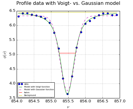
If your profile deviates from a Gaussian shape (e.g. asymmetric profiles) then you can use the so called {it Gauss-Hermite} series. The series are used to derive skewness and kurtosis of your data distribution. The lowest order term of the series is a Gaussian. The higher order terms are orthogonal to this Gaussian. The higher order that we use in our fits are the parameters \(h_3\) and \(h_4\) measuring asymmetric and symmetric deviations of a Gaussian. The Gauss-Hermite function and its applications are described in [Mar], but we use the (equivalent) formulas from [Vog]
with: \(y \equiv \frac{x-\mu_g}{\sigma_g}\).
Simplify this equation further:
or:
with \(E \equiv e^{-\frac{1}{2}y^2}\) and \(Q = \left\{1+h_3(c_1y+c_3y^3)+h_4(c_0+c_2y^2+c_4y^4)\right\}\) and its coefficients:
To find the real maximum (which is not the maximum of the Gaussian part of the expression), solve:
We used SciPy’s function fsolve() in the neighbourhood of 0 to find the solution of this expression.
Moments of the GH series [Vog]
The integrated line strength \(\gamma\):
The mean abscissa \(\mu_{gh}\):
The dispersion \(\sigma_{gh}\):
The Fisher coefficient of Skewness \(\xi_1\):
A set of observations that is not symmetrically distributed is said to be skewed. If the distribution has a longer tail less than the maximum, the function has negative skewness. Otherwise, it has positive skewness.
This is what we could have expected because \(h_3\) is the parameter that measures asymmetric deviations.
The Fisher coefficient of Kurtosis \(\xi_2\):
This parameter measures both the peakedness of the distribution and the heaviness of its tail:
Or use the definition of excess kurtosis \(\xi_f\):
A negative value means that distribution is flatter then a pure Gaussian. and if it is positive then the distribution is sharper then a pure Gaussian. A Gaussian distribution has zero excess kurtosis.
It is obvious that for \(h_3 = 0\) and \(h_4 =0\), all these parameters are the same as their Gaussian counterparts. A line-shape model based on the Gauss-Hermite series will resemble a pure Gaussian. Therefore it is save to set the initial guesses for the \(h_3\) and \(h_4\) parameters in the least-squares fit to zero because. If a fit is successful, the profile parameters \(\gamma_{gh}\), \(\mu_{gh}\) and \(\sigma_{gh}\), skewness and kurtosis are calculated from the best fit parameters \(A\), \(\mu_g\), \(\sigma_{g}\), \(h_3\) and \(h_4\) using the formulas above. For the errors in these parameters we derived:
These formulas are used in the next example. It is a script that finds best-fit parameters of a Gaussian, Voigt and Gauss-Hermite model. Only the last model can quantify the asymmetry of the data. The data is derived from the GH-series and some noise is added. The Voigt line-shape has a problem with asymmetric data. It tends to find negative values for one of the half widths (\(\alpha_D\) or \(\alpha_L\)). To avoid this we use the limits option in kmpfit‘s parinfo dictionary as follows:
>>> fitter.parinfo = [{'limits':(0,None)}, {'limits':(0,None)}, {}, {}, {}]
Example: kmpfit_gausshermite.py - The Gauss-Hermite series compared to Voigt and Gauss
(Source code, png, hires.png, pdf)

Sometimes your data contains errors in both the response (dependent) variable y (i.e. we have values for \(\sigma_y\)) and in the explanatory (independent) variable x (i.e. we have values for \(\sigma_x\)). In the next sections we describe a method to use kmpfit for this category of least squares fit problems.
Assume we have a model function f(x) and on that curve we have a data point \((\hat{x},\hat{y}) = (\hat{x},f(\hat{x}))\) which has the shortest distance to a data point \((x_i,y_i)\). The distance between those points is:
or more general with weights in \(\hat{x},\hat{y}\)
The problem with this distance function is that it is not usable as an Objective Function because we don’t have the model values for \(\hat{x}\). But there is a condition that can be used to express \(\hat{x}\) in known variables \(x_i\) and \(y_i\) Orear [Ore] showed that for any model f(x) for which
is a good approximation, we can find an expression for a usable objective function. \(D_i(\hat{x})\) has a minimum for \(\frac{\partial{D}}{\partial{\hat{x}}} = 0\). Insert (78) in (77) and take the derivative to find the condition for the minimum:
Then one derives:
so that:
If you substitute this in (77), then (after a lot of re-arranging) one finds for the objective function:
If we use statistical weighting with weights \(w_{xi}=1/{\sigma_{xi}}^2\) and \(w_{yi}=1/{\sigma_{yi}}^2\), we can write this as:
The method in the previous section can also be explained in another way: Clutton [Clu] shows that for a model function f, the effect of a small error \(\delta x_i\) in \(x_i\) is to change the measured value \(y_i\) by an amount \(f^\prime (x_i) \delta x_i\) and that as a result, the effective variance of a data point i is:
Equation (83) can be used to create an objective function. We show this for a model which represents a straight line \(f(x)=a+bx\). For a straight line the Taylor approximation (78) is exact. This can be seen as follows: With \(f^\prime(x) = b\). The relation \(f(x) = f(x_i)+(x-x_i)f^{\prime}(x_i)\) is equal to \(f(x) = f(x_i)+(x-x_i)b = a+bx_i+bx-bx_i = a+bx\).
The objective function, chi-square, that needs to be minimized for a straight line is then:
This formula seems familiar. It resembles an ordinary least squares objective function but with ‘corrected’ weights in Y. A suitable residuals function for kmpfit is the square root of this objective function:
def residuals(p, data):
a, b = p
x, y, ex, ey = data
w = ey*ey + b*b*ex*ex
wi = numpy.sqrt(numpy.where(w==0.0, 0.0, 1.0/(w)))
d = wi*(y-model(p,x))
return d
Another approach to find the best fit parameters for orthogonal fits of straight lines starts with the observation that best (unweighted) fitting straight lines for given data points go through the centroid of the system. This applies to regression of y on x, regression of x on y and also for the result of an orthogonal fit.
Note
Unweighted best fitting straight lines for given data points go through the centroid of the system.
If we express our straight line as \(y=b+\tan(\theta)x\) and substitute the coordinates of the centroid \((\bar{x}, \bar{y})\), we get the expression for a straight line:
For a line \(ax+by+c=0\) we know that the distance of a data point \((x_i,y_i)\) to this line is given by: \((ax_i+by_i+c)/\sqrt{(a^2+b^2)}\). If we use this for (86) then we derive an expression for the distance D:
For an objective function we need to minimize:
To minimize this we set the first partial derivative with respect to \(\theta\) to 0 and find the condition:
Fitting problems like the ones we just described are not new. In 1901, Karl Pearson published an article [Pea] in which he discussed a problem “where the Independent Variable is subject to as much deviation or error as the Dependent Variable. He derived the same best-fit angle (89) in a different way (using correlation ellipsoids). Pearson writes it as:
where \(r_{xy}\) is called the Pearson product-moment correlation coefficient. Using the same variables he writes for the slope \(b_1\) of a regression of y on x and the slope \(b_2\) for a regression of x on y:
with:
With (90) and (91) we get the well-known relation between the slopes of the two regression lines and the correlation coefficient:
and (90) can be written as:
On page 571 in this article he presented a table with data points. This table has been used many times in the literature to compare different methods.
>>> x = numpy.array([0.0, 0.9, 1.8, 2.6, 3.3, 4.4, 5.2, 6.1, 6.5, 7.4])
>>> y = numpy.array([5.9, 5.4, 4.4, 4.6, 3.5, 3.7, 2.8, 2.8, 2.4, 1.5])
So let’s prove it works with a short program. The script in the next example calculates Pearson’s best fit slope using the analytical formulas from this section. Then it shows how one can use kmpfit for a regression of y on x and for a regression of x on y. In the latter case, we swap the data arrays x and y in the initialization of kmpfit. Note that for a plot we need to transform its offset and slope in the YX plane to an offset and slope in the XY plane. If the values are \((a,b)\) in the YX plane, then in the XY plane, the offset and slope will be \((-a/b, 1/b)\).
1 2 3 4 5 6 7 8 9 10 11 12 13 14 15 16 17 18 19 20 21 22 23 24 25 26 27 28 29 30 31 32 33 | #!/usr/bin/env python
import numpy
from kapteyn import kmpfit
def model(p, x):
# Model: y = a + numpy.tan(theta)*x
a, theta = p
return a + numpy.tan(theta)*x
def residuals(p, data):
# Residuals function for data with errors in y only
a, b = p
x, y = data
d = (y-model(p,x))
return d
# Pearsons data
x = numpy.array([0.0, 0.9, 1.8, 2.6, 3.3, 4.4, 5.2, 6.1, 6.5, 7.4])
y = numpy.array([5.9, 5.4, 4.4, 4.6, 3.5, 3.7, 2.8, 2.8, 2.4, 1.5])
N = len(x)
fitobj2 = kmpfit.Fitter(residuals=residuals, data=(x, y))
fitobj2.fit(params0=[5,0])
a1, b1 = fitobj2.params[0], numpy.tan(fitobj2.params[1])
fitobj3 = kmpfit.Fitter(residuals=residuals, data=(y, x))
fitobj3.fit(params0=(0,5))
a2, b2 = fitobj3.params[0], numpy.tan(fitobj3.params[1])
tan2theta = 2*b1*b2/(b2-b1)
twotheta = numpy.arctan(tan2theta)
best_slope = numpy.tan(0.5*twotheta)
best_offs = y.mean() - best_slope*x.mean()
print "Best fit parameters: a=%.10f b=%.10f"%(best_offs,best_slope)
|
The most remarkable fact is that Pearson applied the ‘effective variance’ method, formulated at a later date, to an unweighted orthogonal fit, as can be observed in the second plot in the figure. Pearson’s best-fit parameters are the same as the best-fit parameters we find with the effective variance method (look in the output below). In an extended version of the program above, we added the effective variance method and added the offset and slope for the bisector of the two regression lines (y on x and x on y). The results are shown in the next figure. Note that Pearson’s best-fit line is not the same as the bisector which has no relation to orthogonal fitting procedures.
Note
Pearson’s method is an example of an orthogonal fit procedure. It cannot handle weights nor does it give you estimates of the errors on the best-fit parameters. We discussed the method because it is historically important and we wanted to prove that kmpfit can be used for its implementation.
Note
In the example we find best-fit values for the angle \(\theta\) from which we derive the slope \(b = \tan(\theta)\). The advantage of this method is that it also finds fits for data points that represent vertical lines.
Example: kmpfit_Pearsonsdata.py - Pearsons data and method (1901)
(Source code, png, hires.png, pdf)
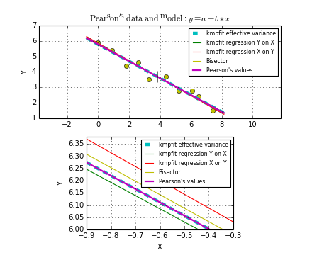
The output of this program is:
1 2 3 4 5 6 7 8 9 10 11 12 13 14 15 16 17 18 19 20 21 22 23 24 25 26 27 28 29 30 31 32 33 34 35 36 | Analytical solution
===================
Best fit parameters: a=5.7840437745 b=-0.5455611975
Pearson's Corr. coef: -0.976475222675
Pearson's best tan2theta, theta, slope: -1.55350214417 -0.49942891481 -0.545561197521
b1 (Y on X), slope: -0.539577274984 -0.539577274984
b2 (X on Y), slope -1.76713124274 -0.565888925403
======== Results kmpfit: effective variance =========
Params: 5.78404377469 -0.545561197496
Covariance errors: [ 0.68291482 0.11704321]
Standard errors [ 0.18989649 0.03254593]
Chi^2 min: 0.618572759437
Reduced Chi^2: 0.0773215949296
======== Results kmpfit Y on X =========
Params: [5.7611851899974615, -0.4948059176648682]
Covariance errors: [ 0.59895647 0.10313386]
Standard errors [ 0.1894852 0.03262731]
Chi^2 min: 0.800663522236
Reduced Chi^2: 0.100082940279
======== Results kmpfit X on Y =========
Params: (10.358385598025167, 5.2273490890768901)
Covariance errors: [ 0.94604747 0.05845157]
Standard errors [ 0.54162728 0.03346446]
Chi^2 min: 2.62219628339
Reduced Chi^2: 0.327774535424
Least squares solution
======================
a1, b1 (Y on X) 5.76118519 -0.539577274869
a2, b2 (X on Y) 5.86169569507 -0.565888925412
Best fit tan2theta, Theta, slope: -1.5535021437 -0.499428914742 -0.545561197432
Best fit parameters: a=5.7840437742 b=-0.5455611974
Bisector through centroid a, b: 5.81116055121 -0.552659830161
|
York [Yor] added weights to Pearsons data. This data set is a standard for comparisons between fit routines for weighted fits. Note that the weights are given as \(w_{x_i}\) which is equivalent to \(1/\sigma_{x_i}^2\).
>>> x = numpy.array([0.0, 0.9, 1.8, 2.6, 3.3, 4.4, 5.2, 6.1, 6.5, 7.4])
>>> y = numpy.array([5.9, 5.4, 4.4, 4.6, 3.5, 3.7, 2.8, 2.8, 2.4, 1.5])
>>> wx = numpy.array([1000.0,1000,500,800,200,80,60,20,1.8,1.0])
>>> wy = numpy.array([1,1.8,4,8,20,20,70,70,100,500])
This standard set is the data we used in the next example. This program compares different methods. One of the methods is the approach of Williamson [Wil] using an implementation described in [Ogr].
Example: kmpfit_Pearsonsdata_compare - Pearson’s data with York’s weights
(Source code, png, hires.png, pdf)

Part of the output of this program is summarized in the next table.
Literature results:
| Reference | a | b |
|---|---|---|
| Pearson unweighted | 5.7857 | -0.546 |
| Williamson | 5.47991022403 | -0.48053340745 |
| Reed | 5.47991022723 | -0.48053340810 |
| Lybanon | 5.47991025 | -0.480533415 |
Practical results:
| Method | a | b |
|---|---|---|
| kmpfit unweighted | 5.76118519259 | -0.53957727555 |
| kmpfit weights in Y only | 6.10010929336 | -0.61081295310 |
| kmpfit effective variance | 5.47991015994 | -0.48053339595 |
| ODR | 5.47991037830 | -0.48053343863 |
| Williamson | 5.47991022403 | -0.48053340745 |
>From these results we conclude that kmpfit with the effective variance residuals function, is very well suited to perform weighted orthogonal fits for a model that represents a straight line. If you run the program, you can observe that also the uncertainties match.
To study the effects of weights and to compare residual functions based on a combination of (81) and (77) and on the effective variance formula in (83) we made a small program which produces random noise for the model data and random weights for the measured data in both x an y. It also compares the results of these methods with SciPy’s ODR routine. If you run the program you will observe that the three methods agree very well.
Example: kmpfit_errorsinXandYPlot - Comparing methods using random weights
(Source code, png, hires.png, pdf)

\(\bf{f([a,b],x) = ax - b/x}\)
We used data from an experiment described in Orear’s article [Ore] to test the effective variance method. Orear starts with a model \(f([a,b],x) = ax - b/x\). He tried to minimize the objective function by an iteration using (80) with the derivative \(f^{\prime}([a,b],x) = a + b/x^2\) and calls this the exact solution. He also iterates using the effective variance method as in (82) and finds small differences between these methods. This must be the result of an insufficient convergence criterion or numerical instability because we don’t find a significant difference using these methods in a program (see example below). The corresponding residual function for the minimum distance expression is:
1 2 3 4 5 6 7 8 9 10 11 12 | def residuals3(p, data):
# Minimum distance formula with expression for x_model
a, b = p
x, y, ex, ey = data
wx = numpy.where(ex==0.0, 0.0, 1.0/(ex*ex))
wy = numpy.where(ey==0.0, 0.0, 1.0/(ey*ey))
df = a + b/(x*x)
# Calculated the approximate values for the model
x0 = x + (wy*(y-model(p,x))*df)/(wx+wy*df*df)
y0 = model(p,x0)
D = numpy.sqrt( wx*(x-x0)**2+wy*(y-y0)**2 )
return D
|
The residual function for the effective variance is:
def residuals(p, data):
# Residuals function for data with errors in both coordinates
a, b = p
x, y, ex, ey = data
w = ey*ey + ex*ex*(a+b/x**2)**2
wi = numpy.sqrt(numpy.where(w==0.0, 0.0, 1.0/(w)))
d = wi*(y-model(p,x))
return d
The conclusion, after running the example, is that kmpfit in combination with the effective variance method finds best-fit parameters that are better than the published best-fit parameters (because a smaller value for the minimum chi-square is obtained). The example shows that for data and model like Orear’s, the effective variance, which includes uncertainties both in x and y, produces a better fit than an Ordinary Least-Squares (OLS) fit where we treat errors in x as being much smaller than the errors in y.
Example: kmpfit_Oreardata - The effective variance method with Orear’s data
(Source code, png, hires.png, pdf)
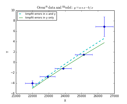
\(\bf{f([a,b,c],x) = ax^2+bx+c}\)
Applying the effective variance method for a parabola we use the objective function:
and we write the following residuals function for kmpfit:
def residuals(p, data):
# Model: Y = a + b*x + c*x*x
a, b, c = p
x, y, ex, ey = data
w = ey*ey + (b+2*c*x)**2*ex*ex
wi = numpy.sqrt(numpy.where(w==0.0, 0.0, 1.0/(w)))
d = wi*(y-model(p,x))
return d
How good is our Taylor approximation here? Using \(f(x) \approx f(x_i)+(x-x_i)(b+2cx_i)\) we find that f(x) can be approximated by: \(f(x) = a + bx + cx^2 - c(x-x_i)^2\). So this approximation works if the difference between \(x_i\) and \(x\) remains small. For kmpfit this implies that also the initial parameter estimates must be of reasonable quality. Using the code of residuals function above, we observed that this approach works adequately. It is interesting to compare the results of kmpfit with the results of Scipy’s ODR routine. Often the results are comparable. That is, if we start with model parameters (a, b, c) = (-6, 1, 0.5) and initial estimates beta0 = (1,1,1), then kmpfit (with smaller tolerance than the default) obtains a smaller value for chi square in 2 of 3 trials. With initial estimates beta0 = (1.8,-0.5,0.1) it performs worse with really wrong fits.
Note
kmpfit in combination with the effective variance method is more sensitive to reasonable initial estimates than Scipy’s ODR.
Example: kmpfit_ODRparabola - The effective variance method for a parabola
(Source code, png, hires.png, pdf)
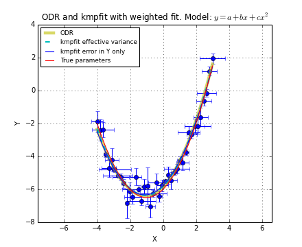
\(\bf{f([a,b,c],x) = a\sin(bx+c)}\)
If your model is not linear in its parameters, then the effective variance method can still be applied. If your model is given for example by \(f(x) = a\sin(bx+c)\), which is not linear in parameter b, then \(f^\prime(x) = ab\cos(bx+c)\) and the effective variance in relation (84) can be implemented as:
1 2 3 4 5 6 7 8 9 10 11 12 13 | def model(p, x):
# Model: Y = a*sin(b*x+c)
a,b,c = p
return a * numpy.sin(b*x+c)
def residuals(p, data):
# Merit function for data with errors in both coordinates
a, b, c = p
x, y, ex, ey = data
w1 = ey*ey + (a*b*numpy.cos(b*x+c))**2*ex*ex
w = numpy.sqrt(numpy.where(w1==0.0, 0.0, 1.0/(w1)))
d = w*(y-model(p,x))
return d
|
In the next script we implemented the listed model and residuals function. The results are compared with SciPy’s ODR routine. The same conclusion applies to these results as to the results of the parabola in the previous section.
Note
kmpfit with effective variance can also be used for models that are not linear in their parameters.
Example: kmpfit_ODRsinus.py - Errors in both variables
(Source code, png, hires.png, pdf)

Experimenters often want to find the best-fit parameters p of their model to predict a value f(p,x) at given x. To get the predicted value \(\hat{y}\) is trivial: \(\hat{y} = f(p,x)\), but to estimate the error in \(\hat{y}\) ( \(\sigma_f)\) is not. Wolberg [Wol] starts with an expression for \(\Delta f\):
which is a Taylor expansion of the error in y neglecting higher order terms. If one repeats the experiment many times, Wolberg finds an expression for the average error \(\bar{{\Delta f}^2}= \sigma^2_f\) in terms of the elements of the covariance matrix:
which implies, as already seen in (96) that this error includes all variances and covariances in the covariance matrix. Note that for unit weighting or relative weighting we need to rescale the covariance matrix elements with \(\chi_{\nu}^2\), and get:
This confidence interval is interpreted as the region in which there is a probability of 68.3% to find the true value of f. To find a confidence region for another probability (e.g. 95%), we need to scale the error using Student-t statistics. If we use \(100(1-\alpha)\) percent to define the confidence interval on any fitted \(\hat{y}_{i}\), then the scale factor is \(t_{\alpha/2, \nu}\). where t is the upper \(\alpha/2\) critical value for the t distribution with N-n degrees of freedom. All the information needed to construct a confidence interval can be found in kpmfit‘s Fitter object:
- Degrees of freedom \(\nu\) = Fitter.dof
- Reduced chi square: \(\chi_{\nu}^2\) = Fitter.rchi2_min
- Covariance matrix: C = Fitter.covar
- Best-fit parameters: p = Fitter.params
Confidence bands are often used in plots to give an impression of the quality of the predictions. To calculate confidence bands we vectorize (98):
which is the short version of:
If your model f is for example a parabola \(f(x) = a + bx +cx^2\), then we have derivatives:
and the confidence band is calculated using:
The next code example shows a function which implements the confidence interval for a given model (variable model is a function or a lambda expression). The list dfdp is a list with derivatives evaluated at the values of x. The values in x need not to be the same values as the x coordinates of your data values. The code uses statistics module stats.t from SciPy to get the critical value for t with method ppf (percent point function). Then with the information in Fitter object fitobj, it creates a NumPy array with the lower values of the confidence interval (lowerband) and an array with the upper values of the confidence interval (upperband).
1 2 3 4 5 6 7 8 9 10 11 12 13 14 15 16 17 18 19 20 21 22 23 24 25 26 27 28 29 30 31 32 33 34 35 36 37 | def confidence_band(x, dfdp, alpha, fitobj, model, abswei):
from scipy.stats import t
# Given the confidence probability confprob = 100(1-alpha)
# we derive for alpha: alpha = 1 - confprob
alpha = 1.0 - confprob
prb = 1.0 - alpha/2
tval = t.ppf(prb, fitobj.dof)
C = fitobj.covar
n = len(fitobj.params) # Number of parameters from covariance matrix
p = fitobj.params
N = len(x)
if abswei:
covscale = 1.0
else:
covscale = fitobj.rchi2_min
df2 = numpy.zeros(N)
for j in range(n):
for k in range(n):
df2 += dfdp[j]*dfdp[k]*C[j,k]
df = numpy.sqrt(fitobj.rchi2_min*df2)
y = f(p, x)
delta = tval * df
upperband = y + delta
lowerband = y - delta
return y, upperband, lowerband
def model(p, x):
# Model: Y = a + b*x + c*x*x
a,b,c = p
return a + b*x + c*x*x
dfdp = [1, x, x**2]
alpha = 0.05
yhat, upperband, lowerband = confidence_band(x, dfdp, alpha, fitobj, model)
|
Confidence bands are plotted in the next program. It uses a 95% confidence probability to draw bands for a fit with weigths in y only and for a fit with errors both in x and y using the effective variance method. We used data and weights, so the weights should be treated as relative weights (abswei=False).
Example: kmpfit_ODRparabola_confidence - Confidence bands fit of parabola
(Source code, png, hires.png, pdf)
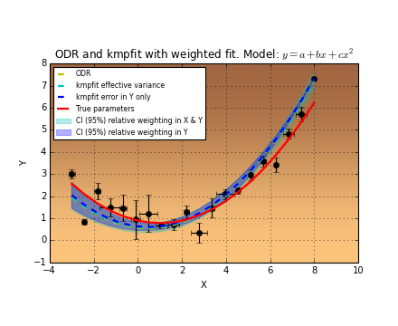
With a small change in the confidence routine we can also derive a prediction interval. The values for a prediction band are derived from:
So we need the array with the data errors to derive the prediction interval. Note that this band is only smooth if we use unit weighting. Otherwise one observes a distorted band due to fluctuations in the weighting as demonstrated on the next example.
Example: kmpfit_example_partialdervs_confidence - Confidence bands fit of parabola
(Source code, png, hires.png, pdf)
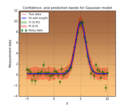
With measurements one often finds one or more data points that appear isolated. If you are convinced that such data is a measurement error then of course you can throw it away or you can use a criterion based on the normal distribution using the (im)probability of large deviations. In this section we discuss a method to remove outliers where a data point is an outlier in the y direction only. The criterion we want discuss here is called Chauvenet’s criterion (http://en.wikipedia.org/wiki/Chauvenet’s_criterion). Suppose you have N measurements \(y_i\) from which we first calculate the mean and standard deviation. If a normal distribution is assumed, we can determine if the probability of a particular measurement is less than 1/2N (as proposed by the French mathematician Chauvenet). So if P is the probability then the criterion is:
In the next example we implemented this criterion to find outliers in a sample. We use the error function scipy.special.erfc() to calculate the probability P in the tails of the normal distribution. We implemented a clear and simple routine and a NumPy based function chauvenet() which is fast and efficient when we need to filter big arrays. This function returns an array of booleans. When an element in that array is False, we reject the corresponding data element in the data arrays:
1 2 3 4 5 6 7 8 9 10 11 12 13 14 15 16 17 18 19 20 21 22 23 24 25 26 27 28 29 30 31 32 33 34 35 36 37 38 39 40 41 42 43 44 | def chauvenet(x, y, mean=None, stdv=None):
#-----------------------------------------------------------
# Input: NumPy arrays x, y that represent measured data
# A single value of a mean can be entered or a
# sequence of means with the same length as
# the arrays x and y. In the latter case, the
# mean could be a model with best-fit parameters.
# Output: It returns a boolean array as filter.
# The False values correspond to the array elements
# that should be excluded
#
# First standardize the distances to the mean value
# d = abs(y-mean)/stdv so that this distance is in terms
# of the standard deviation.
# Then the CDF of the normal distr. is given by
# phi = 1/2+1/2*erf(d/sqrt(2))
# Note that we want the CDF from -inf to -d and from d to +inf.
# Note also erf(-d) = -erf(d).
# Then the threshold probability = 1-erf(d/sqrt(2))
# Note, the complementary error function erfc(d) = 1-erf(d)
# So the threshold probability pt = erfc(d/sqrt(2))
# If d becomes bigger, this probability becomes smaller.
# If this probability (to obtain a deviation from the mean)
# becomes smaller than 1/(2N) than we reject the data point
# as valid. In this function we return an array with booleans
# to set the accepted values.
#
# use of filter:
# xf = x[filter]; yf = y[filter]
# xr = x[~filter]; yr = y[~filter]
# xf, yf are cleaned versions of x and y and with the valid entries
# xr, yr are the rejected values from array x and y
#-----------------------------------------------------------
if mean is None:
mean = y.mean() # Mean of incoming array y
if stdv is None:
stdv = y.std() # Its standard deviation
N = len(y) # Length of incoming arrays
criterion = 1.0/(2*N) # Chauvenet's criterion
d = abs(y-mean)/stdv # Distance of a value to mean in stdv's
d /= 2.0**0.5 # The left and right tail threshold values
prob = erfc(d) # Area normal dist.
filter = prob >= criterion # The 'accept' filter array with booleans
return filter # Use boolean array outside this function
|
In the next example we use the model with the best fit parameters a the mean and the standard deviation of the residuals as the standard deviation for all data points. Note that removing these type of outliers do not change the values of the best-fit parameters much.
Example: kmpfit_chauvenet.py - Exclude bad data with criterion of Chauvenet
(Source code, png, hires.png, pdf)

Another example uses data from [BRo]. A weighted fit gives a value of chi-squared which is too big to accept the hypothesis that the data is consistent with the model. When we use the model and its best-fit parameters as mean and the errors on the data as standard deviation in the function chauvenet(), then one data point is excluded. When we redo the fit, we find a value for chi-squared that is small enough to accept the Null hypothesis that data and model are consistent.
Example: kmpfit_chauvenet2.py - Apply Chauvenet for a weighted fit
(Source code, png, hires.png, pdf)

For outliers in the x direction, one need different methods.
To value a model we use a technique called Variance Reduction [Wol]. It can be applied to both linear and nonlinear models. Variance Reduction (VR) is defined as the percentage of the variance in the dependent variable that is explained by the model. The variance of the sample is given by:
The variance given by the model with its best-fit parameters is:
The Variance Reduction is defined as:
If the quality of your model is good and your data is well behaved, then the model variance is small and the VR is close to 100%. Wrong models, or data with outliers have lower values, which even can be negative. We use VR to identify outliers in data where one (or more) points have a significant error in x. If we calculate the VR for samples where we exclude one data point and repeat this action for all data points, then it is possible to identify the outlier because exclusion of this outlier will improve the VR significantly. Note that for this type of outliers, one cannot use Chauvenet’s criterion because the initial (bad) fit is required to exclude data points.
The VR can be calculated in a script as follows:
fitter.fit(params0=params0) # Find best-fit parameters
varmod = (y-model(fitter.params,x))**2.0 # The model variance
varmod = varmod.sum()/(N-1)
vardat = y.var() # Sample variance
# A vr of 100% implies that the model is perfect
# A bad model gives much lower values (sometimes negative)
vr = 100.0*(1-(varmod/vardat))
Below, the script that uses the VR to identify an outlier. It removes the data point that, when omitted, improves the VR the most.
Example: kmpfit_varreduct.py - Use Variance Reduction to identify outlier
(Source code, png, hires.png, pdf)
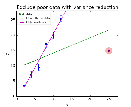
In [Wol] an example is given of data and a fit with using a good model and a bad model. The difference between those models should be clear if we inspect the VR of both. With kmpfit_varreduct_wol.py we reproduced table 3.4.1 of [Wol] for both weighted and unweighted fits. We get the same values, with only a small deviation of the weighted fit with the straight line model ([Wol] gives -48.19, which is probably a typo). The data was derived from a parabolic model so we know that a parabola should be the most suitable model. From the table we learn that indeed the parabola gives the best VR. For weighted fits, the result is even more obvious because the errors on the data increase if the distance from the bottom of the parabola increases. For a weighted fit this is a recipe to get a bad value for the VR.
| Model | \(w_i=1\) | \(w_i=1/\sigma_i^2\) |
|---|---|---|
| \(y = a+b\,x\) | +80.29 | -48.29 |
| \(y = a+b\,x+c\,x^2\) | +99.76 | +99.72 |
Example: kmpfit_varreduct_wol.py - Use Variance Reduction to examine model
(Source code, png, hires.png, pdf)
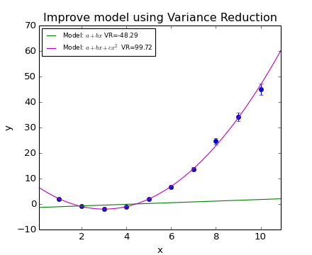
In this section we address a special case of linear regression using an analytical method. It is a regression through the origin. It is used in a practical course where students need to find the Hubble constant after they obtained a number of galaxy velocities and distances. Hubble’s constant can be found if you find the slope of the best fit straight line through the data points (distance in Mpc and velocity in Km/s) and the origin (assuming velocity is zero when the distance is zero).
Hubble’s first fits allowed for an offset and he found an age of the universe that was much too small. Now we know the theoretical base and the fit is reduced to a problem that is known as ‘regression through the origin’.
For a model \(y = a + bx\) we defined chi squared as:
For regression through the origin (leaving parameter a out of the equations) we find for the minimum chi squared:
from which we derive an expression for slope b:
For the standard error in b we follow the procedure described in section Standard errors in weighted fits (20). The error is defined as:
with:
where \(S_{xx}\) does not depend on \(y_i\). With the notation \(S_{xx} = \sum x_i^2 / \sigma_i^2\) we write this as:
Therefore:
Inserting this in (111) gives:
So finally:
In a small program we will demonstrate that this error is the real 1 sigma error for when we exactly know what the errors on the data points are. For weights that are unit or if weights are scaled, we should scale the error on the fitted parameter with the square root of the reduced chi-squared (as described in Reduced chi squared).
The reduced Chi-squared for a regression through the origin is (note we have one parameter less to fit compared to a regression which is not forced to go through the origin):
Then:
This is a two pass algorithm because first you have to find slope b to get the reduced chi-squared. Note that in many references, the unweighted version of the \(\chi_{\nu}^2\) is used to derive the error in slope b. This gives wrong results as can be seen with equal weighting. Many references give the wrong formula, so be careful. A possible implementation of the formulas above is given in the function lingres_origin():
1 2 3 4 5 6 7 8 9 10 11 12 13 | def lingres_origin(xa, ya, err):
# Apply regression through origin
N = len(xa)
w = numpy.where(err==0.0, 0.0, 1.0/(err*err))
sumX2 = (w*xa*xa).sum()
sumXY = (w*xa*ya).sum()
sum1divX = (1/(w*xa)).sum()
b = sumXY/sumX2
sigma_b = 1.0/sumX2
chi2 = (w*(ya-b*xa)**2).sum()
red_chi2 = chi2 / (N-1)
sigma_b_scaled = red_chi2 / sumX2
return b, numpy.sqrt(sigma_b), numpy.sqrt(sigma_b_scaled)
|
Next we show an example of estimating the Hubble constant using data pairs (distance, velocity) found in lab experiments. We use both the analytical method described above and kmpfit to compare the results. We included the fast NumPy based function to filter possible outliers using Chauvenet’s criterion. This criterion was discussed in the previous section. As a mean, we do not use the mean of the sample, but the model with the best fit parameters. As standard deviation we use the (artificial) errors on the data as we did in the second example of Chauvenet’s criterion.
We also included a loop which gives the variance reduction when we omit one data point. The variance reduction for the unfiltered data is low which implies that the model is not the best model or that we have one or more outliers:
1 2 3 4 5 6 7 8 9 10 11 12 13 14 | Variance reduction unfiltered data: 37.38%
Excluded data chi^2 red.chi^2 VR
=====================================================
( 42.00, 1294.00) 32.56 4.65 80.55
( 6.75, 462.00) 101.76 14.54 31.44
( 25.00, 2562.00) 65.93 9.42 41.20
( 33.80, 2130.00) 101.49 14.50 28.46
( 9.36, 750.00) 100.85 14.41 36.82
( 21.80, 2228.00) 75.80 10.83 44.28
( 5.58, 598.00) 99.94 14.28 35.27
( 8.52, 224.00) 99.45 14.21 26.44
( 15.10, 971.00) 101.73 14.53 38.26
=====================================================
|
Based on this table we can conclude that data point (42,1294) can be regarded as an outlier. Removing this point decreases the variance of the data with respect to the model, significantly, which results in a big improvement of the variance reduction. In this case, a filter based on exclusion of data based on variance reduction, improves the fit more than a filter based on Chauvenet’s criterion.
Example: kmpfit_hubblefit.py - Find Hubble constant with fit of line through origin
(Source code, png, hires.png, pdf)

Finding best-fit parameters of an ellipse
In many astronomical problems, the ellipse plays an important role. Examples are planetary orbits, binary star orbits, projections of galaxies onto the sky. etc. For an overview of ellipse properties and formulas, please visit Wolfram’s page about ellipses at http://mathworld.wolfram.com/Ellipse.html Assume we got a number of measurements of the orbit of a binary system and all sky positions are converted to a rectangular grid positions (i.e. x,y coordinate pairs). If one makes a plot of these positions it is usually obvious if have to deal with an elliptical orbit. To estimate typical orbit parameters (e.g. in Kepler’s laws of planetary motion) we have to estimate the best-fit ellipse parameters. These parameters are the position of the center of the ellipse, the length of the major and minor axes and the position angle (its rotation). If we want to fit ellipse parameters we have to find a suitable relation between y and x first. The equation for an unrotated ellipse with semi-major axis a and semi-minor axis b is:
Rotation of the ellipse follows the mathematical standard, i.e. an angle is positive if it is counted anti-clockwise. So if we want an expression for a rotated ellipse we use the rotation recipe:
If the origin is not centered at position (0,0) then we need a translation also:
Introduce a new function Z which depends on variables x and y.
This function is plotted in the surface plot below. The ellipse in this landscape can be found at a height 1.0. We projected the ellipse on the xy plane to prove that the two contours correspond. You can run the example and rotate the 3D plot to get an impression of the landscape. For a data position \((x,y)\) which is exactly on the ellipse \(Z(x,y) = 1\). But if not, then \(Z(x,y)\) deviates from 1.0 and it is a measure for the deviations we are trying to minimize with a least squares fit. Note that the values in \((x,y)\) represents the data on the ellipse. So in fact the should be written as \((x'',y'')\). To calculate \(Z(x,y)\), we need to calculate \((x',y')\) first and from those coordinates the values of \((x,y)\).
In the code example at the end of this section we need a list with positions that we want to use to make a fit. The data we used can be found in ellipse.dat. It is data from an artificial ellipse with origin at (5,4) semi-major axis is 10, semi-minor axis is 3. Its angle is 60 degrees. Noise was added to simulate real data.
But usually we don’t know about the properties of the ellipse represented by the data so we need a routine that calculates these estimates automatically. For the ellipse there is a method based on image moments analysis (http://en.wikipedia.org/wiki/Image_moments) that can do the job.
The zeroth and first moments for the given set data points (positions) are given by:
In an image the zeroth moment represents the area of an object. For our positions \((x,y)\) it is just the number of positions. Note that our data points are just positions and not image pixels with an intensity. So the value of f is 1 for a position from the file and 0 for others (but there are no others because we don’t have an image, just the values in \((x,y)\). Therefore we need only to loop over all our positions and do the necessary summing. Then the coordinates of the centroid (center of mass) are:
which is an estimate of the central position of the ellipse. How can we find an estimate for the other parameters? First we define the so called central moments of the sample:
Now define:
With these definitions, one can derive the following relations:
\(\theta\) gives us estimate for the angle and \(\lambda_i\) the (squared) length of the semi-major and semi-minor axes. We implemented these relations in a routine that finds initial estimates of the parameters of an ellipse based on the moments analysis above:
1 2 3 4 5 6 7 8 9 10 11 12 13 14 15 16 17 18 19 20 21 22 23 24 25 26 27 28 29 30 31 32 | def getestimates( x, y ):
"""
Method described in http://en.wikipedia.org/wiki/Image_moments
in section 'Raw moments' and 'central moments'.
Note that we work with scalars and not with arrays. Therefore
we use some functions from the math module because the are
faster for scalars
"""
m00 = len(x)
m10 = numpy.add.reduce(x)
m01 = numpy.add.reduce(y)
m20 = numpy.add.reduce(x*x)
m02 = numpy.add.reduce(y*y)
m11 = numpy.add.reduce(x*y)
Xav = m10/m00
Yav = m01/m00
mu20 = m20/m00 - Xav*Xav
mu02 = m02/m00 - Yav*Yav
mu11 = m11/m00 - Xav*Yav
theta = (180.0/numpy.pi) * (0.5 * atan(-2.0*mu11/(mu02-mu20)))
if (mu20 < mu02): # mu20 must be maximum
(mu20,mu02) = (mu02,mu20) # Swap these values
theta += 90.0
d1 = 0.5 * (mu20+mu02)
d2 = 0.5 * sqrt( 4.0*mu11*mu11 + (mu20-mu02)**2.0 )
maj = sqrt(d1+d2)
min = sqrt(d1-d2)
return (Xav, Yav, maj, min, theta)
|
If you study the code of the next example, you should be able to recognize the formulas we used in this section to get initial estimates and residuals. The applied method can be used for many fit problems related to 2D data.
Example: kmpfit_ellipse.py - Find best-fit parameters of ellipse model
(Source code, png, hires.png, pdf)

| [Alp] | Alper, Joseph S., Gelb, Robert I., Standard Errors and Confidence Intervals in Nonlinear Regression: Comparison of Monte Carlo and Parametric Statistics, J. Phys. Chem., 1990, 94 (11), pp 4747–4751 (Journal of Physical Chemistry) |
| [And] | Andrae, R, Error estimation in astronomy: A guide, arXiv:1009.2755v3 [astro-ph.IM] 29 Oct 2010 |
| [Bev] | (1, 2) Bevington, Philip R. , Data Reduction and Error Analysis for the Physical Sciences, 1969, McGraw-Hill |
| [BRo] | Bevington, P.R., Robinson D.K., Data Reduction and Error Analysis for the Physical Sciences, Version 2.0 RLM (23 August 2003) |
| [Clu] | Clutton-Brock, Likelihood Distributions for Estimating Functions When Both Variables Are Subject to Error, Technometrics, Vol. 9, No. 2 (May, 1967), pp. 261-269 |
| [Ds1] | DeSerio, R., Statistical Analysis of Data for PHY48803L, Advanced Physics Laboratory, University of Florida (version 1) Local copy: statmain-florida.pdf |
| [Ds2] | DeSerio, R., Statistical Analysis of Data for PHY48803L, Advanced Physics Laboratory, University of Florida (version 2) Local copy: statmain.pdf |
| [Ds3] | (1, 2) DeSerio, R., Regression Algebra, Local copy: matproof_statmain.pdf |
| [Mar] | Marel, P. van der, Franx, M., A new method for the identification of non-gaussian line profiles in elliptical galaxies. A.J., 407 525-539, 1993 April 20 |
| [Mas] | Massey, F. J. The Kolmogorov-Smirnov Test for Goodness of Fit., Journal of the American Statistical Association, Vol. 46, No. 253, 1951, pp. 68-78 |
| [Mkw] | Markwardt, C. B. 2008, “Non-Linear Least Squares Fitting in IDL with MPFIT,” in proc. Astronomical Data Analysis Software and Systems XVIII, Quebec, Canada, ASP Conference Series, Vol. 411, eds. D. Bohlender, P. Dowler & D. Durand (Astronomical Society of the Pacific: San Francisco), p. 251-254 (ISBN: 978-1-58381-702-5) Website: http://purl.com/net/mpfit |
| [Num] | (1, 2, 3, 4) William H. Press, Saul A. Teukolsky, William T. Vetterling and Brian P. Flannery, Numerical Recipes in C, The Art of Scientific Computing, 2nd edition, Cambridge University Press, 1992 |
| [Ogr] | Ogren, J., Norton, J.R., Applying a Simple Linear Least-Squares Algorithm to Data with Uncertainties in Both Variables, J. of Chem. Education, Vol 69, Number 4, April 1992 |
| [Ore] | (1, 2) Orear, Jay, Least squares when both variables have uncertainties, Am. J. Phys. 50(10), Oct 1982 |
| [Pea] | Pearson, K. On lines and planes of closest fit to systems of points in space. Philosophical Magazine 2:559-572, 1901. A copy of this article can be found at: http://stat.smmu.edu.cn/history |
| [Scr] | (1, 2) Schreier, Franz, Optimized implementations of rational approximations for the Voigt and complex error function, Journal of Quantitative Spectroscopy & Radiative Transfer 112 (2011) 1010-1025 |
| [Sch] | (1, 2, 3) Schwarz, U.J., Analysis of an Observed Function into Components, using its Second Derivative, Bull. Astr. Inst. Netherlands, 1968, 19 405-413 (local copy) |
| [Sha] | Shao, J., Jackknifing Weighted Least Squares Estimators, Journal of the Royal Statistical Society. Series B (Methodological), Vol. 51, No. 1(1989), pp. 139-156 |
| [Yor] | York, D. Least-squares fitting of a straight line, Canadian Journal of Physics. Vol. 44, p.1079, 1966 |
| [Vog] | (1, 2, 3, 4) Vogelaar, M.G.R., XGAUPROF, local copy |
| [Wil] | Williamson, Least-squares fitting of a straight line, J.A., Can. J. Phys, 1968, 46, 1845-1847 |
| [Wol] | (1, 2, 3, 4, 5, 6) Wolberg, J., Data Analysis Using the Method of Least Squares, 2006, Springer |
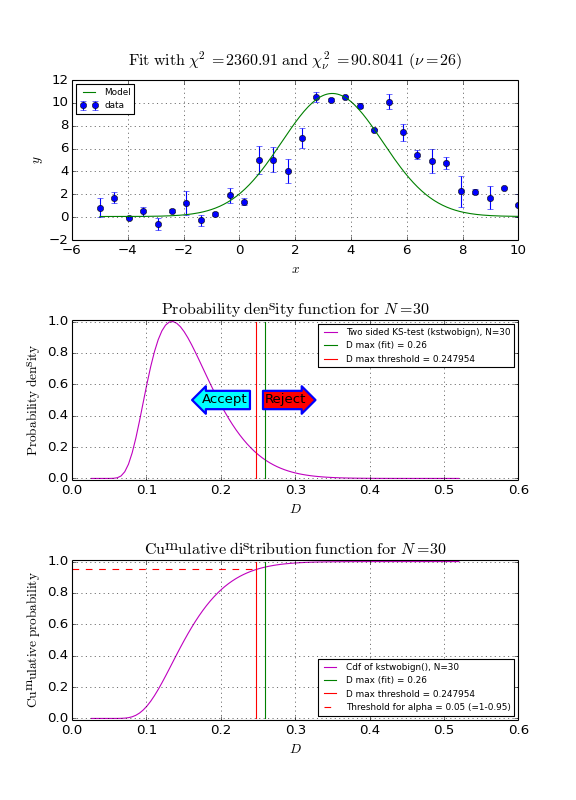
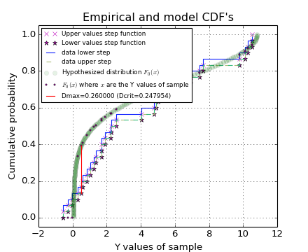
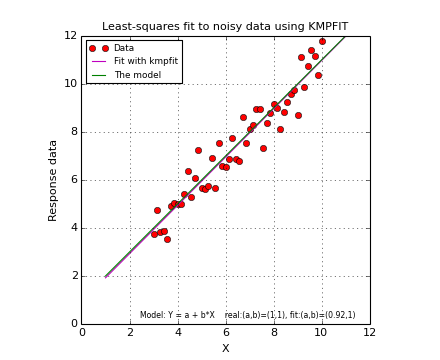
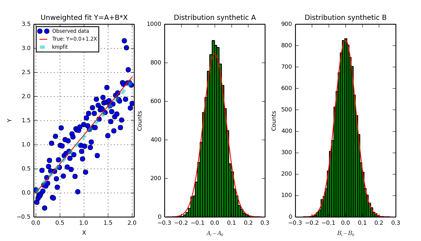
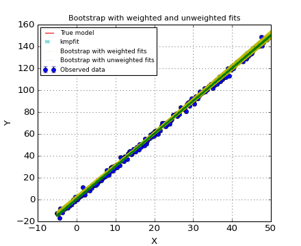
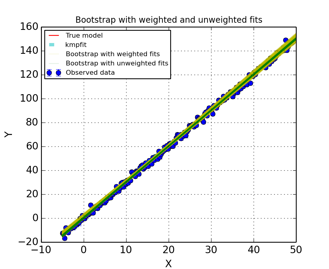
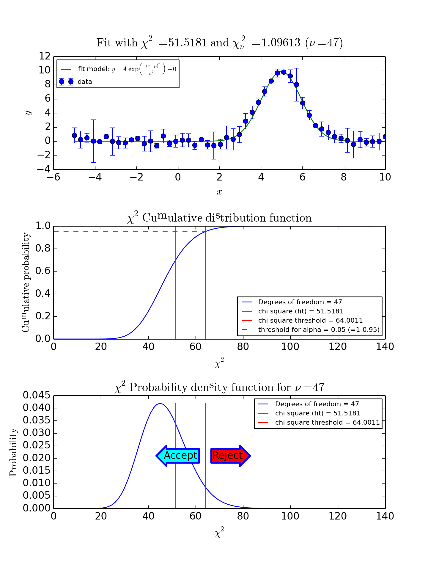
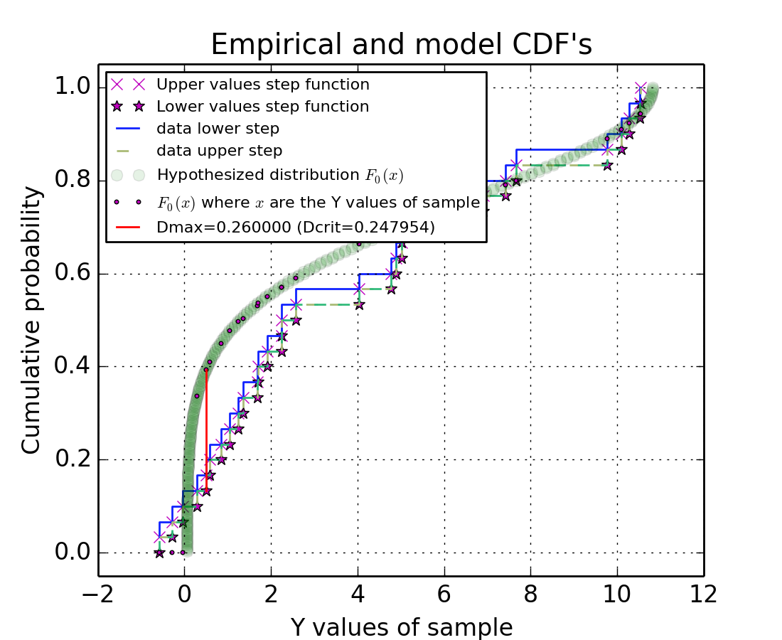
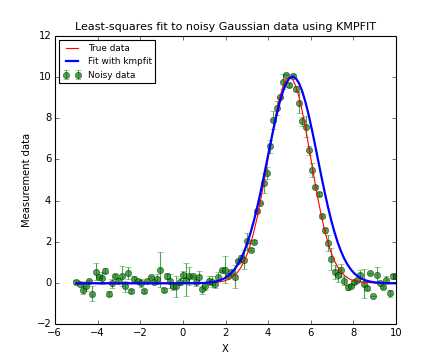
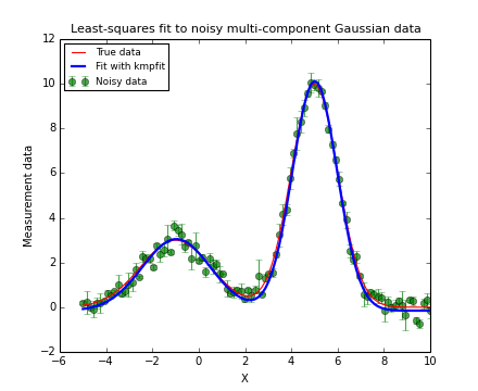
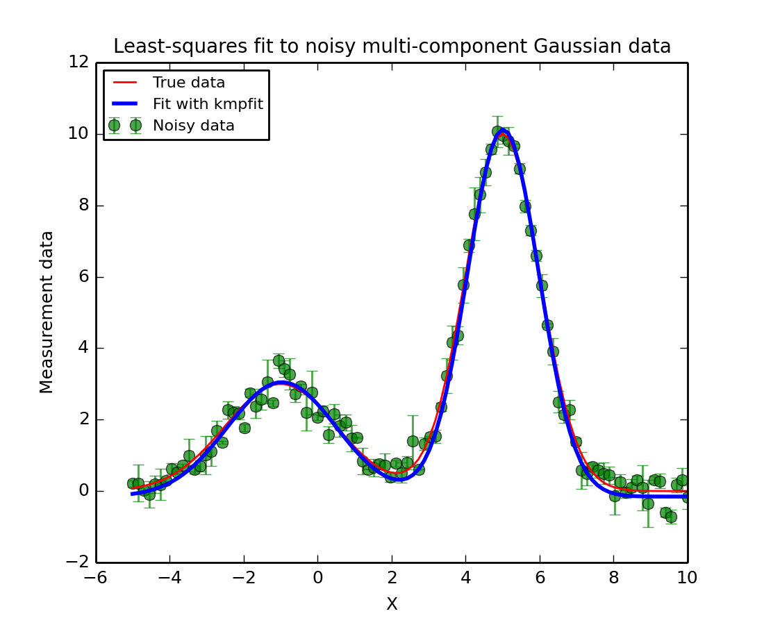
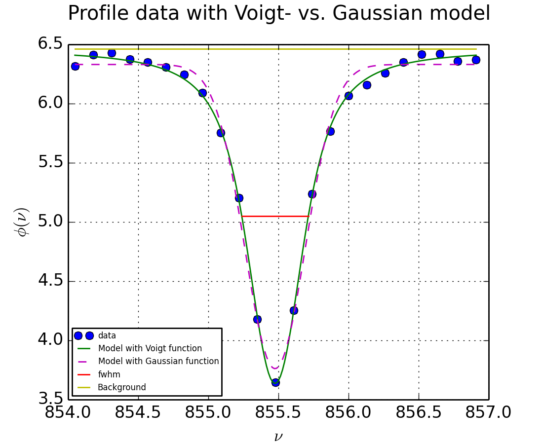
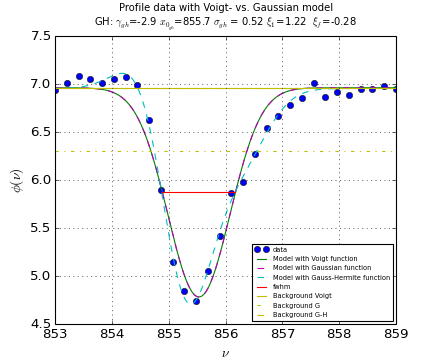
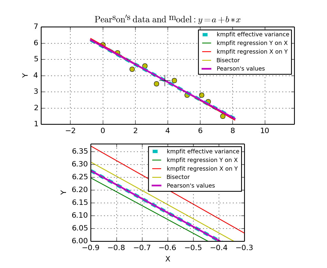
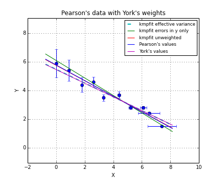
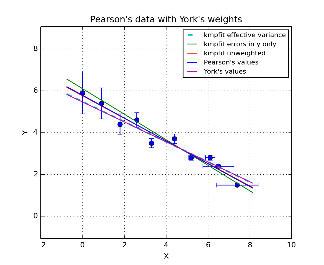
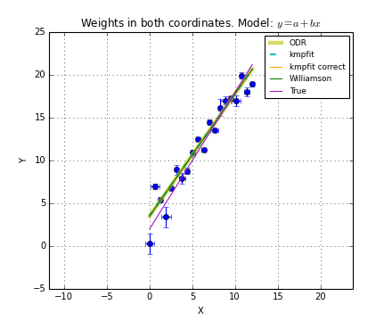
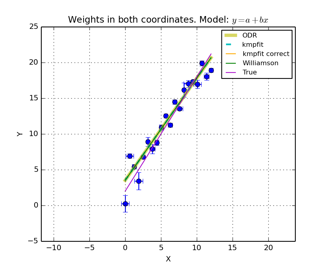
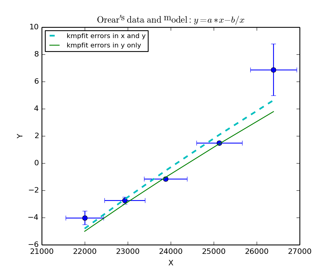
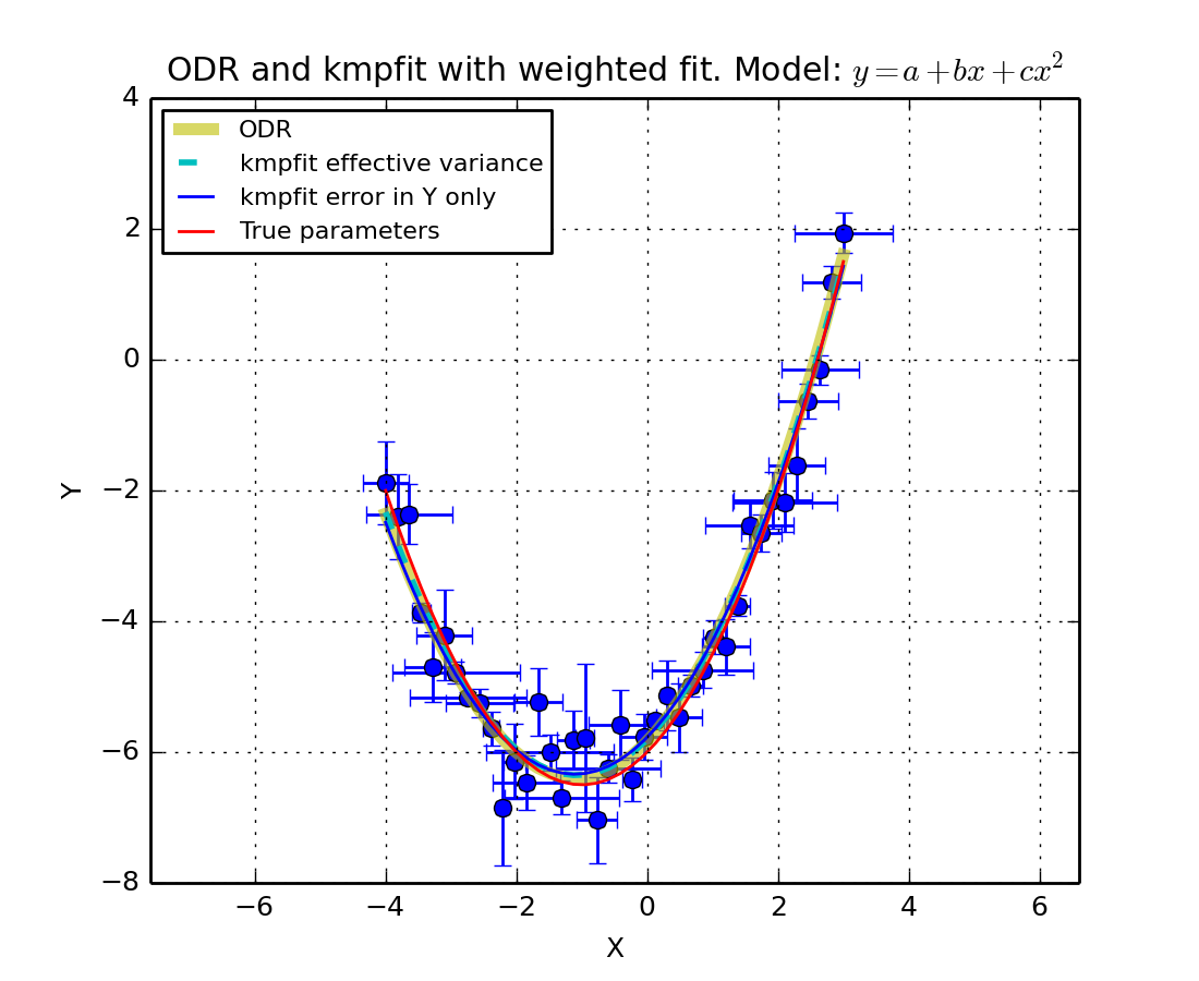
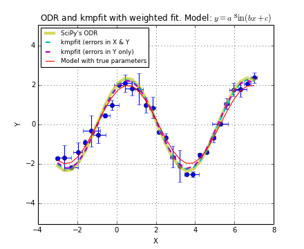
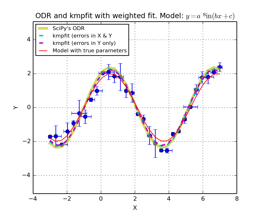
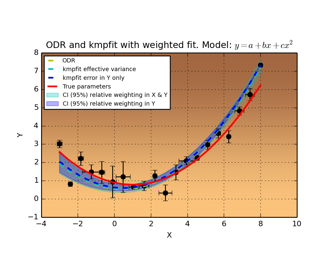
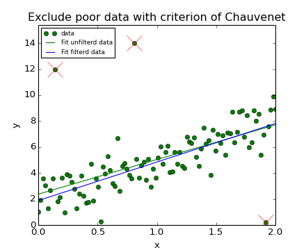
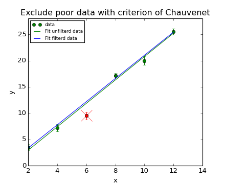
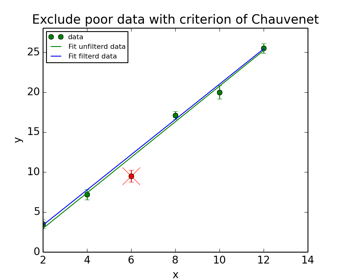
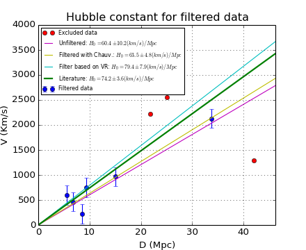
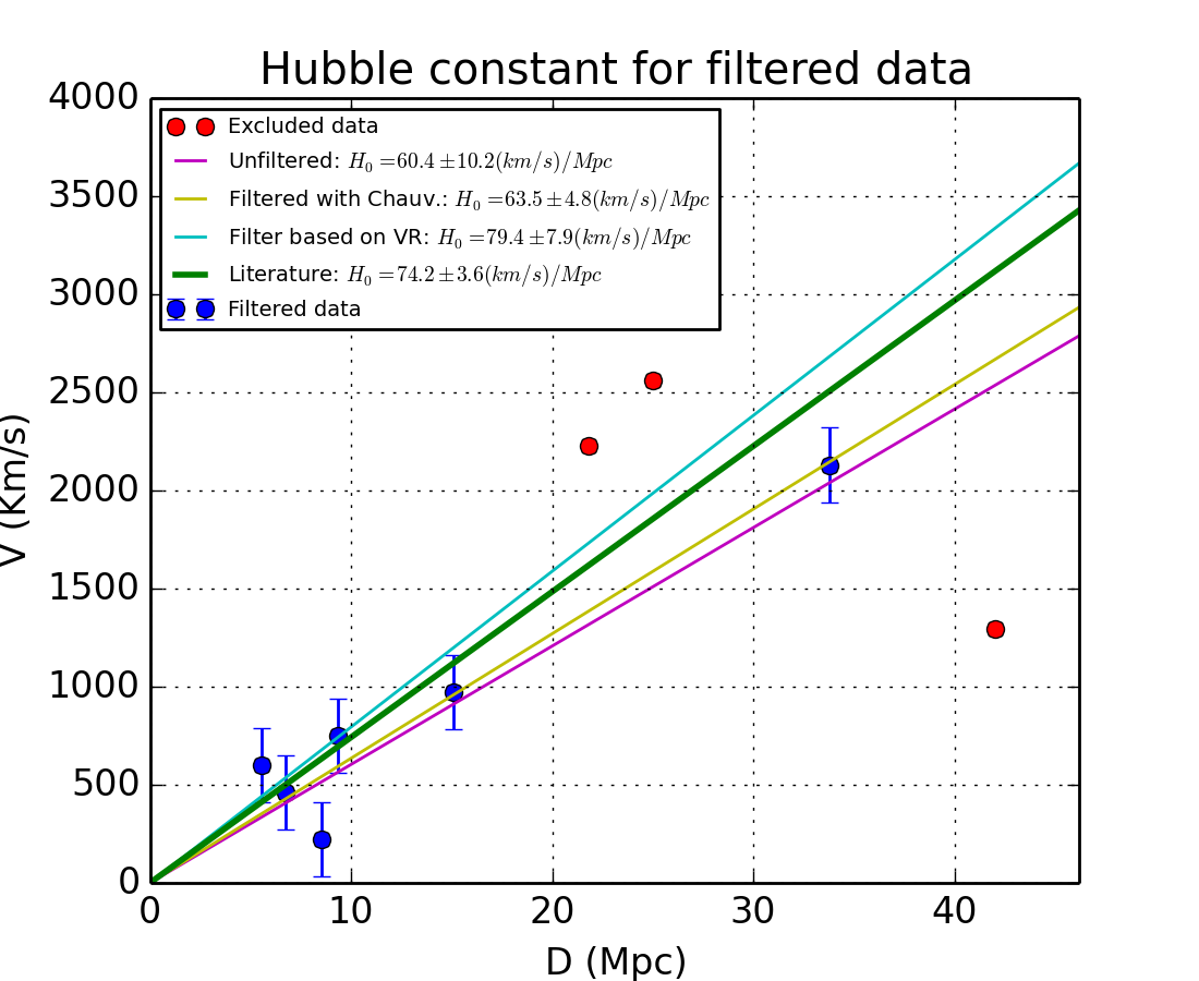
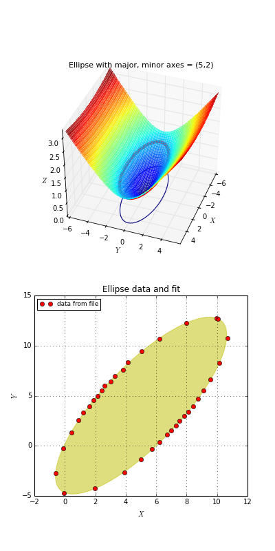
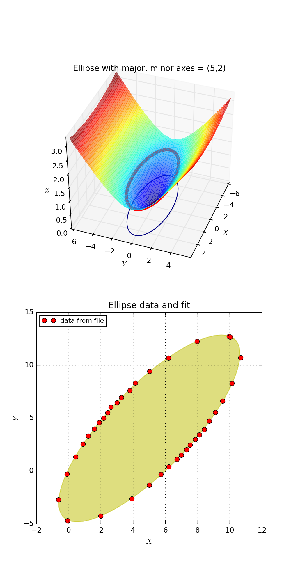