All sky plots and graticules
All Sky plots
An all sky plot is a plot where the range in longitude is
[0,360> and the range in latitude is [-90,90>.
There are many examples in Calabretta’s article
Representations of celestial coordinates in FITS
We tried to reproduce these figures both to prove that the modules in the Kapteyn Package
have the functionality to do it and to facilitate users who want to set up
an all-sky plot with module maputils. For this purpose we
created for each figure the minimal required FITS headers.
Header and other code is listed below the examples.
In the HTML documentation, click on the hires link to get a plot which shows more details.
With the information in this document, it should be easy to compose
a Python program that creates just a single plot which then can be
enhanced to fit your needs.
The first plot is a stand alone version. The others are generated with
different Python scripts and the service module
service.py
(see also the source code at the end of this document).
from kapteyn import maputils
from numpy import arange
from matplotlib import pyplot as plt

dec0 = 89.9999999999   # Avoid plotting on the wrong side
header = {'NAXIS'  :  2,
          'NAXIS1' :  100, 'NAXIS2': 80,
          'CTYPE1' : 'RA---TAN',
          'CRVAL1' :  0.0, 'CRPIX1' : 50, 'CUNIT1' : 'deg',
          'CDELT1' : -5.0, 'CTYPE2' : 'DEC--TAN',
          'CRVAL2' :  dec0, 'CRPIX2' : 40,
          'CUNIT2' : 'deg', 'CDELT2' : 5.0,
         }
X = arange(0,360.0,15.0)
Y = [20, 30,45, 60, 75]

fig = plt.figure(figsize=(7,6))
frame = fig.add_axes((0.1,0.1,0.8,0.8))
f = maputils.FITSimage(externalheader=header)
annim = f.Annotatedimage(frame)
grat = annim.Graticule(wylim=(20.0,90.0), wxlim=(0,360),
                       startx=X, starty=Y)
grat.setp_gratline(color='0.75')
lon_world = list(range(0,360,30))
lat_world = [20, 30, 60, 90]
grat.setp_lineswcs1(20, color='g', linestyle='--')

# Plot labels inside the plot
lon_constval = None
lat_constval = 20
lon_kwargs = {'color':'r', 'fontsize':15}
lat_kwargs = {'color':'b', 'fontsize':10}
grat.Insidelabels(wcsaxis=0,
                  world=lon_world, constval=lat_constval,
                  fmt="Dms",
                  **lon_kwargs)
grat.Insidelabels(wcsaxis=1,
                  world=lat_world, constval=lon_constval,
                  fmt="Dms",
                  **lat_kwargs)
annim.plot()
# Set title for Matplotlib
titlepos = 1.02
title = r"Gnomonic projection (TAN) diverges at $\theta=0^\circ$. (Cal. fig.8)"
t = frame.set_title(title, color='g')
t.set_y(titlepos)
plt.show()
(Source code, png, hires.png, pdf)
The recipe
The next session shows a gallery of all sky plots, all based on the same recipe.
One starts with a self-made header which ensures a complete coverage of the sky by stretching the values of the
CDELT’s.Then an object from class
maputils.Annotatedimage.Graticuleis created with explicit limits for the world coordinates in both directions.For these plots we don’t have intersections of the graticule with an enclosing rectangle so we cannot plot standard axis labels for the coordinates. Instead we use method
wcsgrat.Graticule.Insidelabels()to plot labels inside the plot. In the plots we show different examples how one can manipulate these labeling.
All sky plot gallery
In the title of the plots we refer to the figure numbers in Calabretta’s article Representations of celestial coordinates in FITS. These references start with the abbreviation Cal..
Note that the labels along the enclosing plot rectangle only indicate the types for the longitude and latitude axes and their main direction.
The code which was used to produce a figure is listed just above the plot.
If you want to reproduce a plot then you need this source and the
service module
service.py.
For plots where it is possible to plot a marker at position (120 deg, 60 deg)
we plot a small circle with: annim.Marker(pos=markerpos, marker='o', color='red')
This code is part of the service module
service.py
Note that positions in parameter pos in method maputils.Annotatedimage.Marker()
can be entered in different formats. Have a look at positions for examples.
Definitions
The definitions in this section are consistent with [Ref2] and [Ref2] but simplified. For the FITS keywords we ommitted the suffix for the axis number and the alternate header description (e.g. as in CRVAL2Z).
CTYPE : Type of celestial system and projection system
CRPIX : Pixel coordinate of a coordinate reference point
CRVAL : The world coordinate at the reference point
CDELT : World coordinate increment at the reference point
CUNIT : Units of the world coordinates. For celestial coordinates the required units are ‘deg’. However for wcs/WCSLIB the following lines are equal, because the units are parsed and converted to degrees if necessary:
'CRVAL1' : 120.0*60, 'CRPIX1' : 50, 'CUNIT1' : 'arcmin', 'CDELT1' : 5.0*60
'CRVAL1' : 120.0, 'CRPIX1' : 50, 'CUNIT1' : 'deg', 'CDELT1' : 5.0CROTA : Usually the angle in degrees between the axis for which CROTA is given and the direction of the North. Rotations can also be included in the FITS CD or PC matrix.
The pixel position that corresponds to the values of CRPIX is denoted with \((r_x, r_y)\).
An arbitrary pixel coordinate is denoted with \((p_x, p_y)\).
If we apply an operation M involving the PC or CD matrix or CDELT and CROTA we get \(X = M.(p-r)\). The result is a position denoted with \((x, y)\) and its coordinates are called intermediate world coordinates and in this context we refer to them as projection plane coordinates.
The coordinate reference point is at \((x, y) = (0, 0)\).
Intermediate coordinates are in degrees.
PV FITS cards have syntax \(PVi\_na\) i.e. the keyword starts with PV, it is associated with axis i, it has a number n and can be part of an alternate header identified by a. The PV elements are called coordinate parameters and are used to change the default coordinate system.
With the projection information in CTYPE one converts projection plane coordinates \((x, y)\) to native longitude and latitude, \((\phi, \theta)\). Additional information for this transformation can be given in FITS PV keywords.
Native longitude and latitude \((\phi, \theta)\) are transformed to celestial coordinates \((\alpha, \delta)\) using the world coordinates (CRVAL) of the reference point.
The coordinates of the reference point given by CRVAL is denoted with \((\alpha_0, \delta_0)\) If we assume that a longitude axis is associated with axis 1 in in the FITS file and latitude with axis 2 then \((\alpha_0, \delta_0) = (CRVAL1, CRVAL2)\).
\((\alpha_0, \delta_0)\) is associated with the native longitude and latitude reference point \((\phi_0, \theta_0)\)
This \((\phi_0, \theta_0)\) depends on the projection or its values are given in FITS PV keywords. With the previous assumption of the axis order, these elements will be \(PV1_1\) and \(PV1_2\)
For the transformation from native longitude and latitude \((\phi, \theta)\) to celestial coordinates we need the native longitude and latitude of the celestial pole \((\phi_p, \theta_p)\). Either defaults are taken or values are copied from FITS keywords LONPOLE, LATPOLE or PV1_3 and PV1_4. Also we need the celestial position of the native pole \((\alpha_p, \delta_p)\). (and \(\delta_p = \theta_p\) ).
We summarize what can be varied in the FITS headers we used to plot all sky graticules.
\((\alpha_0, \delta_0) \leftrightarrow (CRVAL1, CRVAL2)\)
native longitude and latitude of reference point \((\phi_0, \theta_0) \leftrightarrow (PV1\_1, PV1\_2)\)
native latitude of the celestial pole \((\phi_p, \theta_p) \leftrightarrow (LONPOLE, LATPOLE) \leftrightarrow (PV1\_3, PV1\_4)\)
In certain classes of projections \((\alpha_0, \delta_0)\) is decoupled from the reference point. To restore the relation between FITS cards CRVALn and CRPIXn one can use PVi_0 where i is the axis number of the longitude axis. Any value unequal to 0.0 will do the job.
Standard versus Oblique
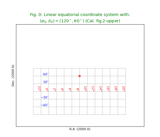
Fig.0: Linear equatorial coordinate system
Before the non-linear coordinate transformations, world coordinates were calculated in a linear way using the number of pixels from the reference point in CRPIX times the increment in world coordinate and added to that the value of CRVAL. We demonstrate this system by creating a header where we omitted the code in CTYPE that sets the projection system.
WCSLIB does not recognize a valid projection system and defaults to linear transformations.
The header is a Python dictionary. With method maputils.Annotatedimage.Graticule() we draw
the graticules. The graticule lines that we want to draw are given by their start position
startx= and starty=. The labels inside the plot are set by lon_world and lat_world.
To be consistent with fig.2 in Cal. [Ref2] , we inserted a positive CDELT for the longitude.
Note
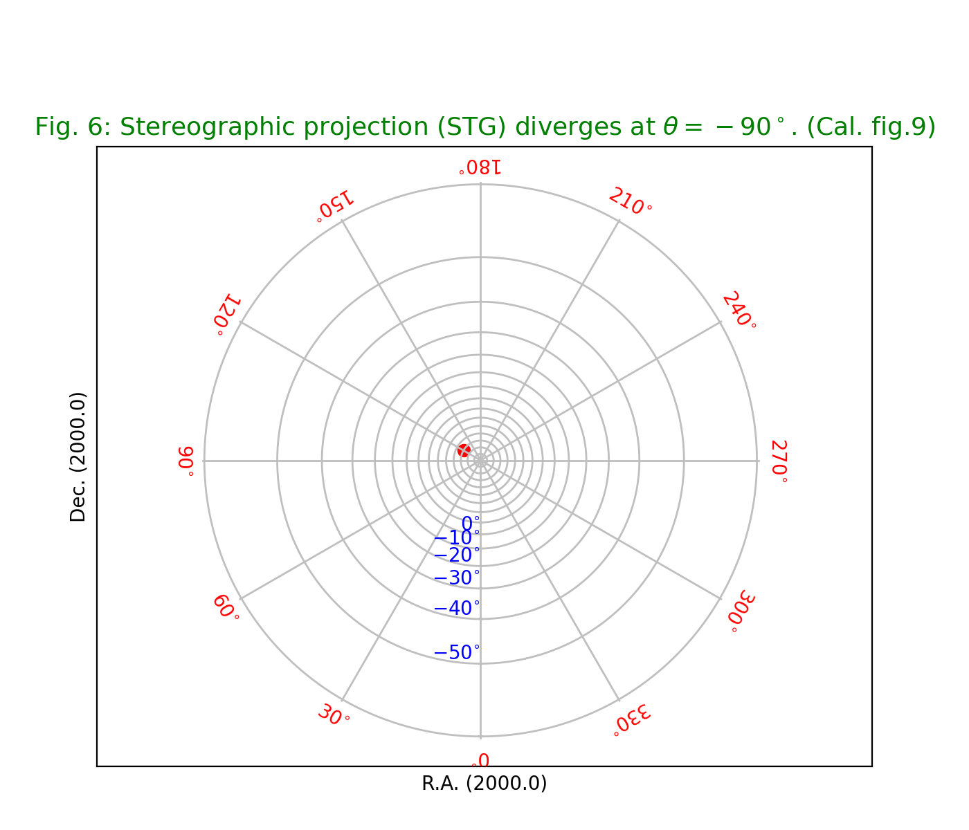
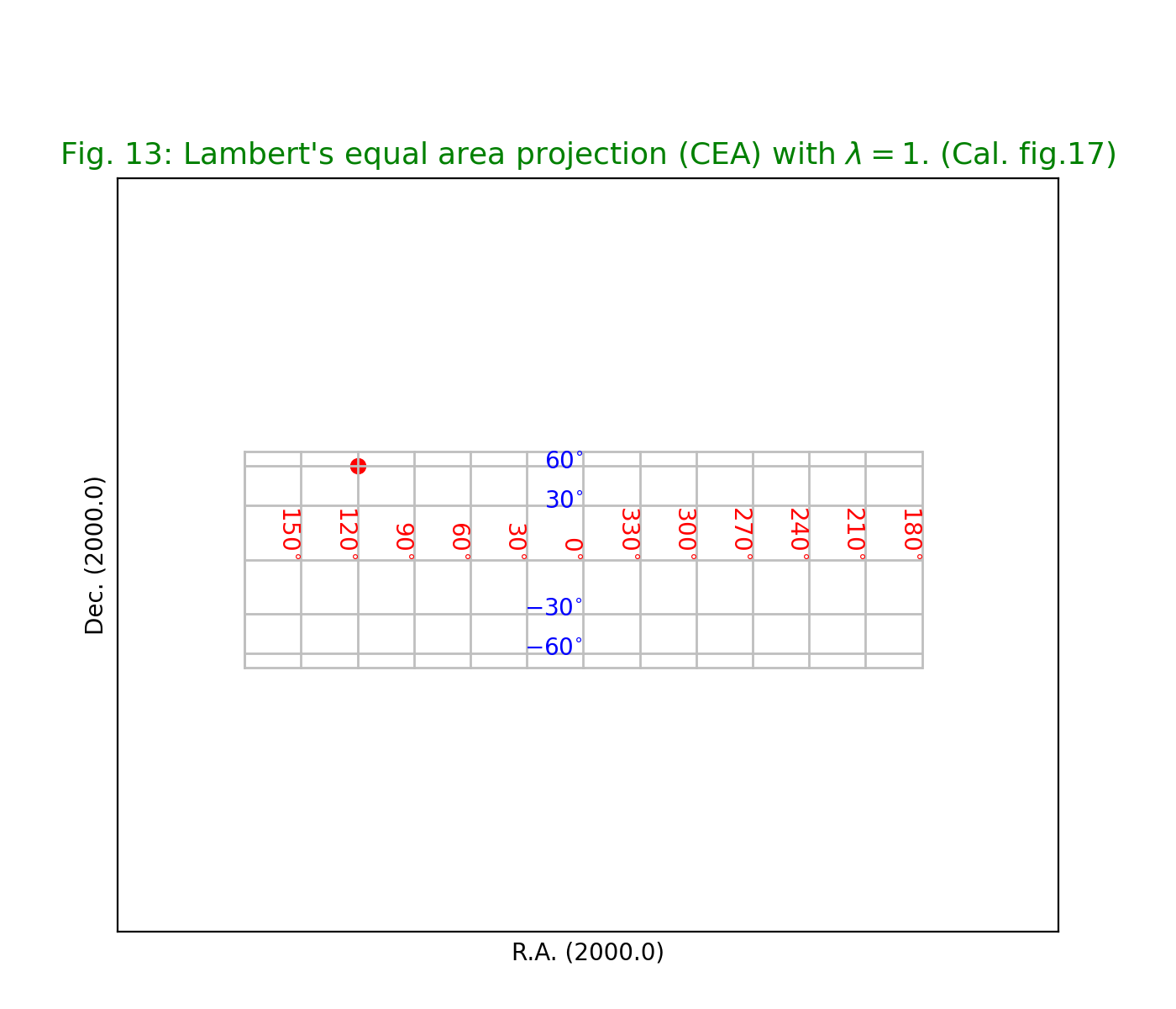
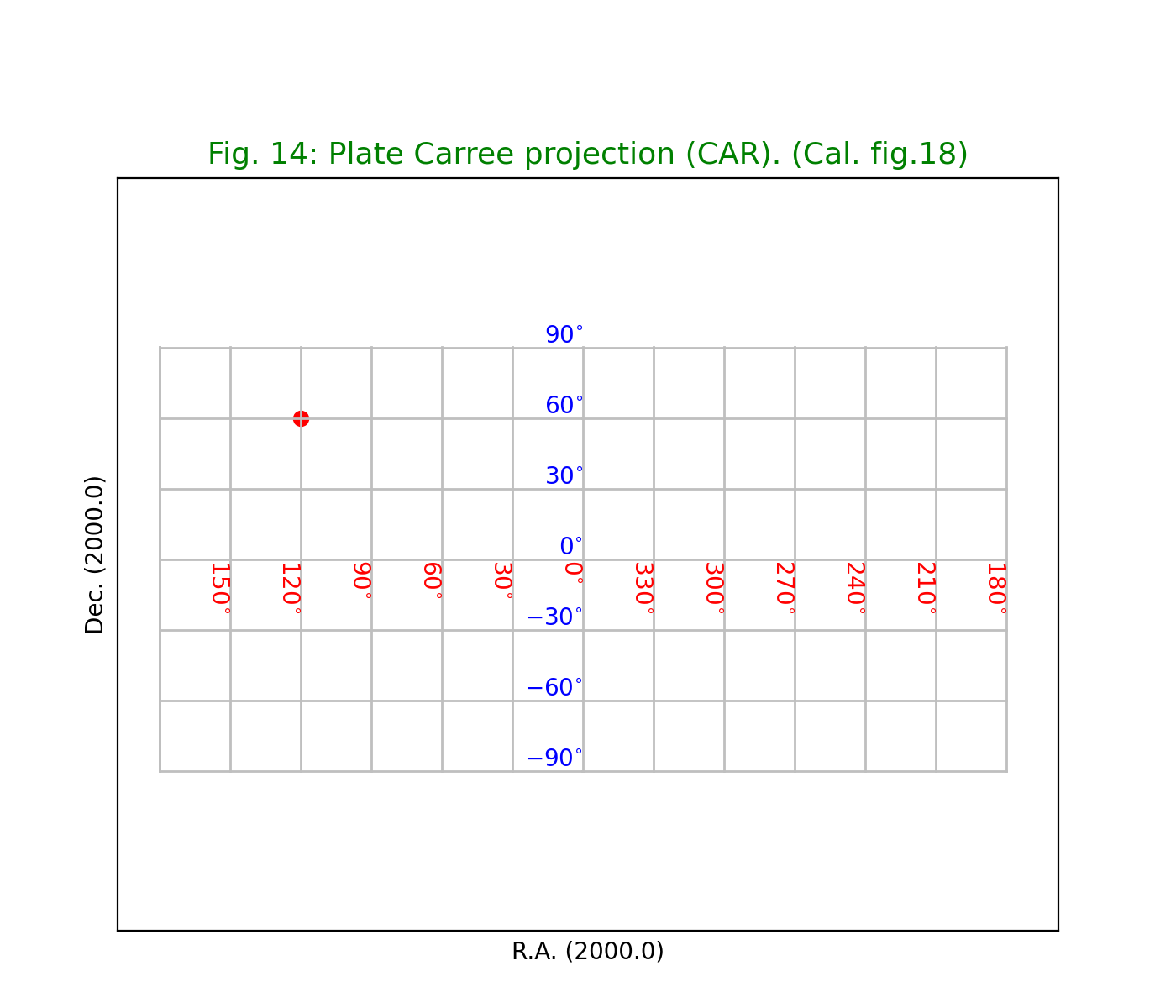
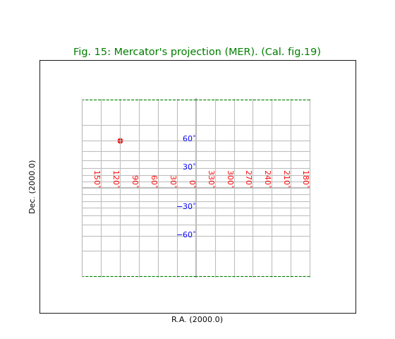
In most of the figures in this section we plot position \((120^\circ,60^\circ)\) as a small solid red circle.
from kapteyn import maputils
import numpy
from service import *

# Fig 2 in celestial article (Calabretta et al) shows a  positive cdelt1
fignum = 0                   # id of script and plot
fig = plt.figure(figsize=figsize)
frame = fig.add_axes(plotbox)
title = r"""Linear equatorial coordinate system with:
$(\alpha_0,\delta_0) = (120^\circ,60^\circ)$ (Cal. fig.2-upper)"""
header = {'NAXIS'  : 2, 'NAXIS1': 100, 'NAXIS2': 80,
          'CTYPE1' : 'RA',
          'CRVAL1' : 120.0, 'CRPIX1' : 50, 'CUNIT1' : 'deg', 'CDELT1' : 5.0,
          'CTYPE2' : 'DEC',
          'CRVAL2' : 60.0, 'CRPIX2' : 40, 'CUNIT2' : 'deg', 'CDELT2' : 5.0,
         }
X = numpy.arange(-60,301.0,30.0);
Y = numpy.arange(-90,100,30.0)  # i.e. include +90 also
f = maputils.FITSimage(externalheader=header)
annim = f.Annotatedimage(frame)
grat = annim.Graticule(header, axnum=(1,2),
                       wylim=(-90,90.0), wxlim=(-60,300),
                       startx=X, starty=Y)
#print "Lonpole, latpole values: ", \
#      annim.projection.lonpole, annim.projection.latpole,
lat_world = [-60, -30, 30, 60]
lon_world = list(range(-30,301,30))
labkwargs0 = {'color':'r', 'va':'bottom', 'ha':'right'}
labkwargs1 = {'color':'b', 'va':'bottom', 'ha':'right'}
doplot(frame, fignum, annim, grat, title,
       lat_world=lat_world, lon_world=lon_world,
       lon_fmt='Hms',
       labkwargs0=labkwargs0, labkwargs1=labkwargs1,
       markerpos=markerpos)
(Source code, png, hires.png, pdf)

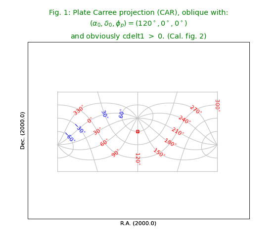
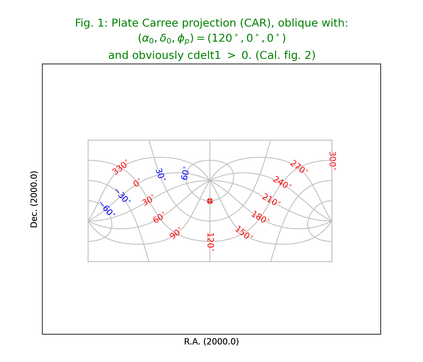
Fig.1: Oblique Plate Carree projection (CAR)
In [Ref2] we read that only CTYPE needs to be changed to get the next figure.
For CTYPE the projection code CAR is added. For a decent plot we need to draw a border.
The trick for plotting borders for oblique versions is to change header values
to the non-oblique version and then to draw only the limiting graticule lines.
In method maputils.Annotatedimage.Graticule()
we use parameters startx and starty to specify these limits as in:
startx=(180-epsilon,-180+epsilon), starty=(-90,90))
This plot shows an oblique version. A problem with oblique all sky plots is drawing a closed border. The trick that we applied a number of times is to overlay the border of the non-oblique version.
from kapteyn import maputils
import numpy
from service import *

# Fig 2 in celestial article (Calabretta et al) shows a  positive cdelt1
fignum = 1
fig = plt.figure(figsize=figsize)
frame = fig.add_axes(plotbox)
title = r"""Plate Carree projection (CAR), oblique with:
$(\alpha_0,\delta_0,\phi_p) = (120^\circ,0^\circ,0^\circ)$
and obviously cdelt1 $>$ 0. (Cal. fig. 2)"""
header = {'NAXIS'  : 2, 'NAXIS1': 100, 'NAXIS2': 80,
          'CTYPE1' : 'RA---CAR',
          'CRVAL1' : 120.0, 'CRPIX1' : 50, 'CUNIT1' : 'deg', 'CDELT1' : 5.0,
          'CTYPE2' : 'DEC--CAR',
          'CRVAL2' : 60.0, 'CRPIX2' : 40, 'CUNIT2' : 'deg', 'CDELT2' : 5.0,
          'LONPOLE' : 0.0,
         }
X = numpy.arange(0,360.0,30.0)
Y = numpy.arange(-60,80,30.0)

f = maputils.FITSimage(externalheader=header)
annim = f.Annotatedimage(frame)
grat = annim.Graticule(header, axnum= (1,2),
                       wylim=(-90,90.0), wxlim=(0,360),
                       startx=X, starty=Y)

# Get the non-oblique version for the border
header['CRVAL1'] = 0.0
header['CRVAL2'] = 0.0
border = annim.Graticule(header, axnum= (1,2),
                         wylim=(-90,90.0), wxlim=(-180,180),
                         startx=(180-epsilon,-180+epsilon), starty=(-90,90))
lat_world = [-60, -30, 30, 60]
doplot(frame, fignum, annim, grat, title,
       lat_world=lat_world, deltapx1=0, deltapy1=0,
       markerpos=markerpos)
(Source code, png, hires.png, pdf)

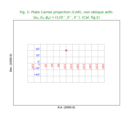
Fig.2: Plate Carree projection non-oblique (CAR)
To get a non oblique version of the previous system we need to change the value of \(\delta_0\) (as given in CRVAL2) to 0 because for this projection \(\phi_p = 0\). In the header we changed CRVAL2 to 0.
from kapteyn import maputils
import numpy
from service import *

# Fig 2 in celestial article (Calabretta et al) shows a  positive cdelt1
fignum = 2                   # id of script and plot
fig = plt.figure(figsize=figsize)
frame = fig.add_axes(plotbox)
title = r"""Plate Carree projection (CAR), non oblique with:
$(\alpha_0,\delta_0,\phi_p) = (120^\circ,0^\circ,0^\circ)$. (Cal. fig.2)"""
header = {'NAXIS'  : 2, 'NAXIS1': 100, 'NAXIS2': 80,
          'CTYPE1' : 'RA---CAR',
          'CRVAL1' : 120.0, 'CRPIX1' : 50, 'CUNIT1' : 'deg', 'CDELT1' : 5.0,
          'CTYPE2' : 'DEC--CAR',
          'CRVAL2' : 0.0, 'CRPIX2' : 40, 'CUNIT2' : 'deg', 'CDELT2' : 5.0,
          'LONPOLE': 0.0
         }
X = numpy.arange(0,380.0,30.0);
Y = numpy.arange(-90,100,30.0)  # i.e. include +90 also
f = maputils.FITSimage(externalheader=header)
annim = f.Annotatedimage(frame)
grat = annim.Graticule(header, axnum=(1,2),
                       wylim=(-90,90.0), wxlim=(0,360),
                       startx=X, starty=Y)
header['CRVAL1'] = 0.0
border = annim.Graticule(header, axnum=(1,2),
                         wylim=(-90,90.0), wxlim=(-180,180),
                         startx=(180-epsilon,-180+epsilon, 0),
                         starty=(-90,0,90))
lat_world = list(range(-60, 61, 30))
lon_world = list(range(-30,301,30))
labkwargs0 = {'color':'r', 'va':'top', 'ha':'right'}
labkwargs1 = {'color':'b', 'va':'bottom', 'ha':'right'}
doplot(frame, fignum, annim, grat, title,
       lat_world=lat_world, lon_world=lon_world,
       labkwargs0=labkwargs0, labkwargs1=labkwargs1,
       markerpos=markerpos)
(Source code, png, hires.png, pdf)

Zenithal projections
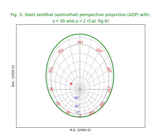
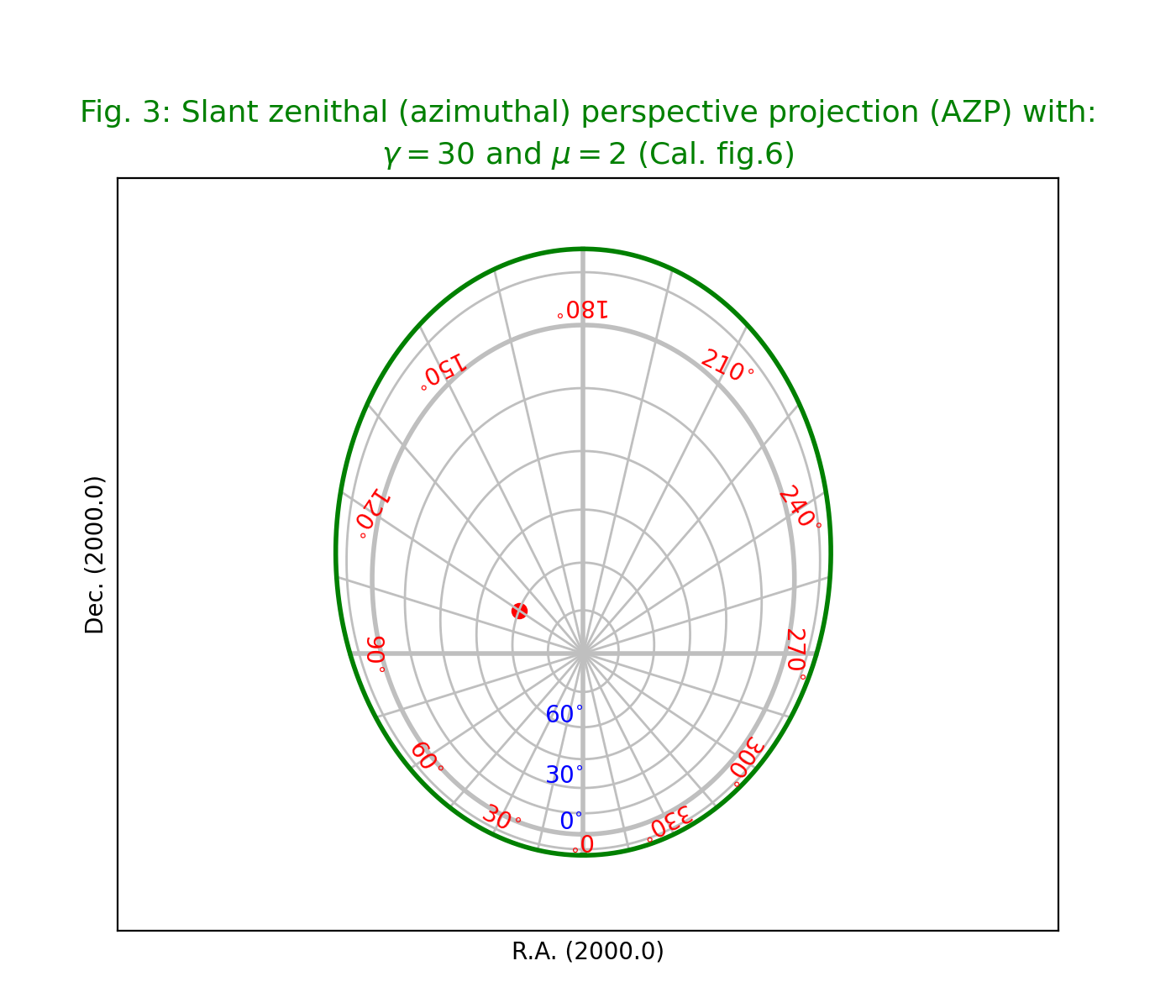
Fig.3: Slant zenithal (azimuthal) perspective projection (AZP)
This figure shows a projection for which we need to specify extra
parameters in the so called PV header keywords as in:
'PV2_1' : mu, 'PV2_2' : gamma
It uses a formula given in Calabretta’s article to get a value for the border:
lowval = (180.0/numpy.pi)*numpy.arcsin(-1.0/mu) + 0.00001
from kapteyn import maputils
import numpy
from service import *

fignum = 3
fig = plt.figure(figsize=figsize)
frame = fig.add_axes(plotbox)
mu = 2.0; gamma = 30.0
title = r"""Slant zenithal (azimuthal) perspective projection (AZP) with:
$\gamma=30$ and $\mu=2$ (Cal. fig.6)"""
header = {'NAXIS' : 2, 'NAXIS1': 100, 'NAXIS2': 80,
          'CTYPE1' : 'RA---AZP',
          'CRVAL1' :0, 'CRPIX1' : 50, 'CUNIT1' : 'deg', 'CDELT1' : -4.0,
          'CTYPE2' : 'DEC--AZP',
          'CRVAL2' : dec0, 'CRPIX2' : 30, 'CUNIT2' : 'deg', 'CDELT2' : 4.0,
          'PV2_1'  : mu, 'PV2_2'  : gamma,
         }
lowval = (180.0/numpy.pi)*numpy.arcsin(-1.0/mu) + 0.00001  # Calabretta eq.32
X = numpy.arange(0,360,15.0)
Y = numpy.arange(-30,89,15.0);
Y[0] = lowval                    # Add lowest possible Y to array
f = maputils.FITSimage(externalheader=header)
annim = f.Annotatedimage(frame)
grat = annim.Graticule(axnum=(1,2),
                       wylim=(lowval,90.0), wxlim=(0,360),
                       startx=X, starty=Y)
grat.setp_lineswcs0((0,90,180,270), lw=2)
grat.setp_lineswcs1(0, lw=2)
grat.setp_lineswcs1(lowval, lw=2, color='g')
lat_world = [0, 30, 60, 90]
lon_world = list(range(0,360,30))
labkwargs0 = {'color':'r', 'va':'center', 'ha':'center'}
labkwargs1 = {'color':'b', 'va':'bottom', 'ha':'right'}
addangle0 = -90
lat_constval= -5
doplot(frame, fignum, annim, grat, title,
       lon_world=lon_world, lat_world=lat_world,
       lat_constval=lat_constval,
       labkwargs0=labkwargs0, labkwargs1=labkwargs1,
       addangle0=addangle0, markerpos=markerpos)
(Source code, png, hires.png, pdf)

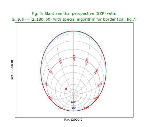
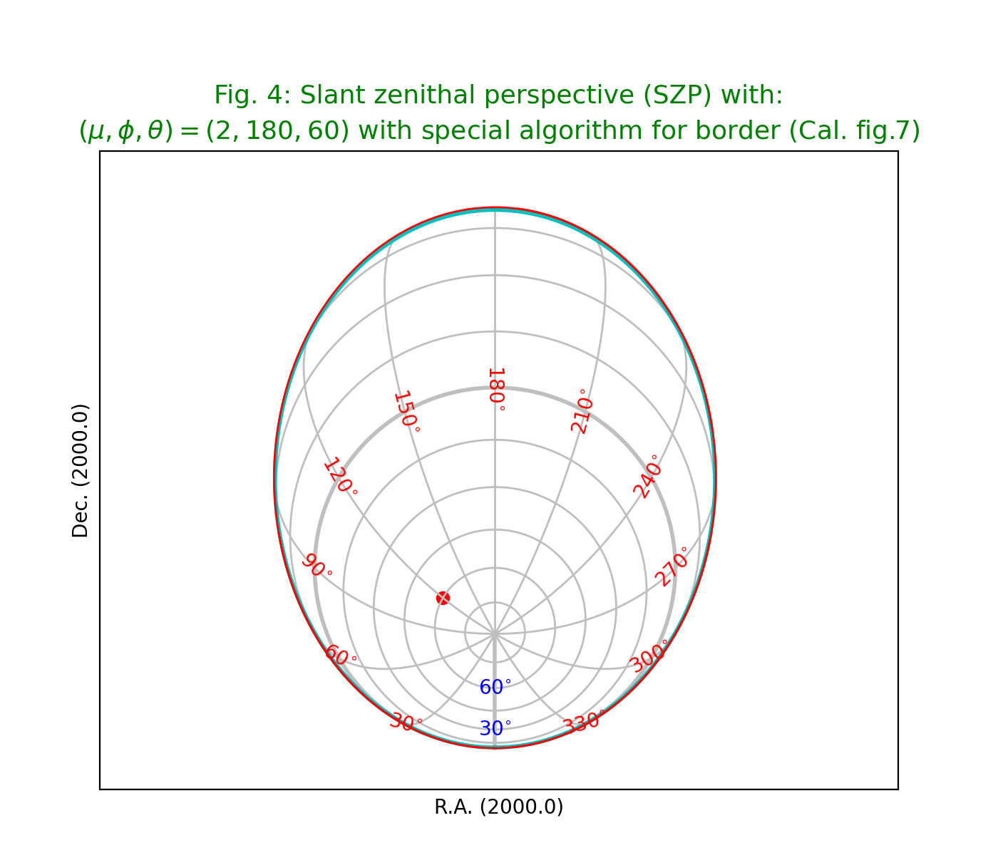
Fig.4: Slant zenithal perspective (SZP)
The plot shows two borders. We used different colors to distinguish them.
The cyan colored border is calculated with a border formula given in [Ref2] and the
red border is calculated with a brute force method wcsgrat.Graticule.scanborder()
which uses a bisection method in X and Y direction to find the position
of a transition between a valid world coordinate and an invalid coordinate.
Obviously the border that is plotted according to the algorithm is less accurate.
The brute force method gives a more accurate border but needs the user to
enter start positions for the bisection.
from kapteyn import maputils
import numpy
from service import *

fignum = 4
fig = plt.figure(figsize=figsize)
frame = fig.add_axes(plotbox)
mu = 2.0; phi = 180.0; theta = 60
title = r"""Slant zenithal perspective (SZP) with:
($\mu,\phi,\theta)=(2,180,60)$ with special algorithm for border (Cal. fig.7)"""
header = {'NAXIS' : 2, 'NAXIS1': 100, 'NAXIS2': 80,
          'CTYPE1' : 'RA---SZP',
          'CRVAL1' : 0.0, 'CRPIX1' : 50, 'CUNIT1' : 'deg', 'CDELT1' : -4.0,
          'CTYPE2' : 'DEC--SZP',
          'CRVAL2' : dec0, 'CRPIX2' : 20, 'CUNIT2' : 'deg', 'CDELT2' : 4.0,
          'PV2_1'  : mu, 'PV2_2'  : phi, 'PV2_3' : theta,
         }
X = numpy.arange(0,360.0,30.0)
Y = numpy.arange(-90,90,15.0)
f = maputils.FITSimage(externalheader=header)
annim = f.Annotatedimage(frame)
grat = annim.Graticule(axnum=(1,2),
                       wylim=(-90.0,90.0), wxlim=(-180,180),
                       startx=X, starty=Y)

grat.setp_lineswcs0(0, lw=2)
grat.setp_lineswcs1(0, lw=2)
# Special care for the boundary
# The algorithm seems to work but is not very accurate
xp = -mu * numpy.cos(theta*numpy.pi/180.0)* numpy.sin(phi*numpy.pi/180.0)
yp =  mu * numpy.cos(theta*numpy.pi/180.0)* numpy.cos(phi*numpy.pi/180.0)
zp =  mu * numpy.sin(theta*numpy.pi/180.0) + 1.0
a = numpy.linspace(0.0,360.0,500)
arad = a*numpy.pi/180.0
rho = zp - 1.0
sigma = xp*numpy.sin(arad) - yp*numpy.cos(arad)
sq = numpy.sqrt(rho*rho+sigma*sigma)
omega = numpy.arcsin(1/sq)
psi = numpy.arctan2(sigma,rho)
thetaxrad = psi - omega
thetax = thetaxrad * 180.0/numpy.pi + 5
g = grat.addgratline(a, thetax, pixels=False)
grat.setp_linespecial(g, lw=2, color='c')
# Select two starting points for a scan in pixel to find borders
g2 = grat.scanborder(68.26,13,3,3)
g3 = grat.scanborder(30,66.3,3,3)
grat.setp_linespecial(g2, color='r', lw=1)
grat.setp_linespecial(g3, color='r', lw=1)
lon_world = list(range(0,360,30))
lat_world = [-60, -30, 30, 60, 90]
#labkwargs0 = {'color':'r', 'va':'center', 'ha':'center'}
#labkwargs1 = {'color':'b', 'va':'bottom', 'ha':'right'}

doplot(frame, fignum, annim, grat, title,
       lon_world=lon_world, lat_world=lat_world,
#       labkwargs0=labkwargs0, labkwargs1=labkwargs1,
       markerpos=markerpos)
(Source code, png, hires.png, pdf)

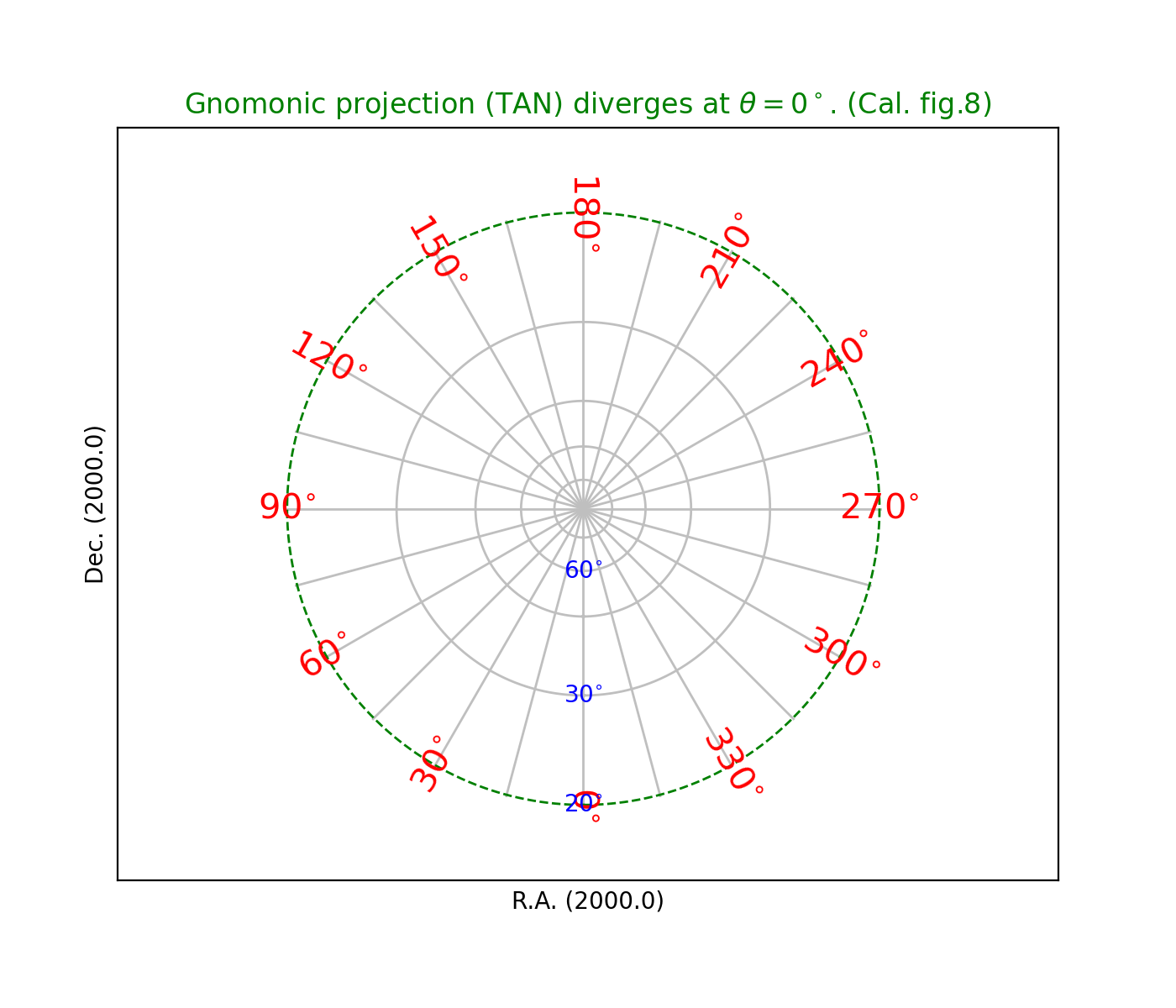
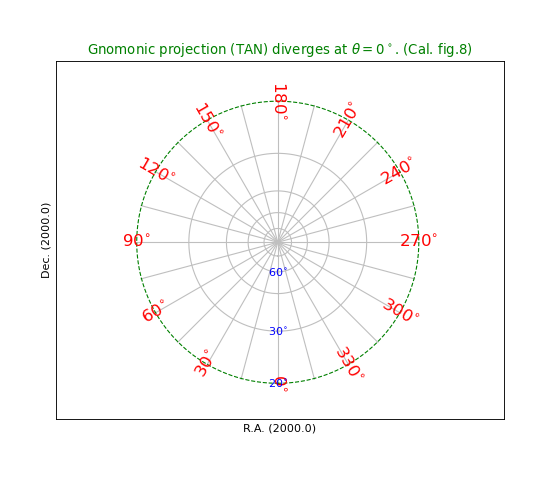
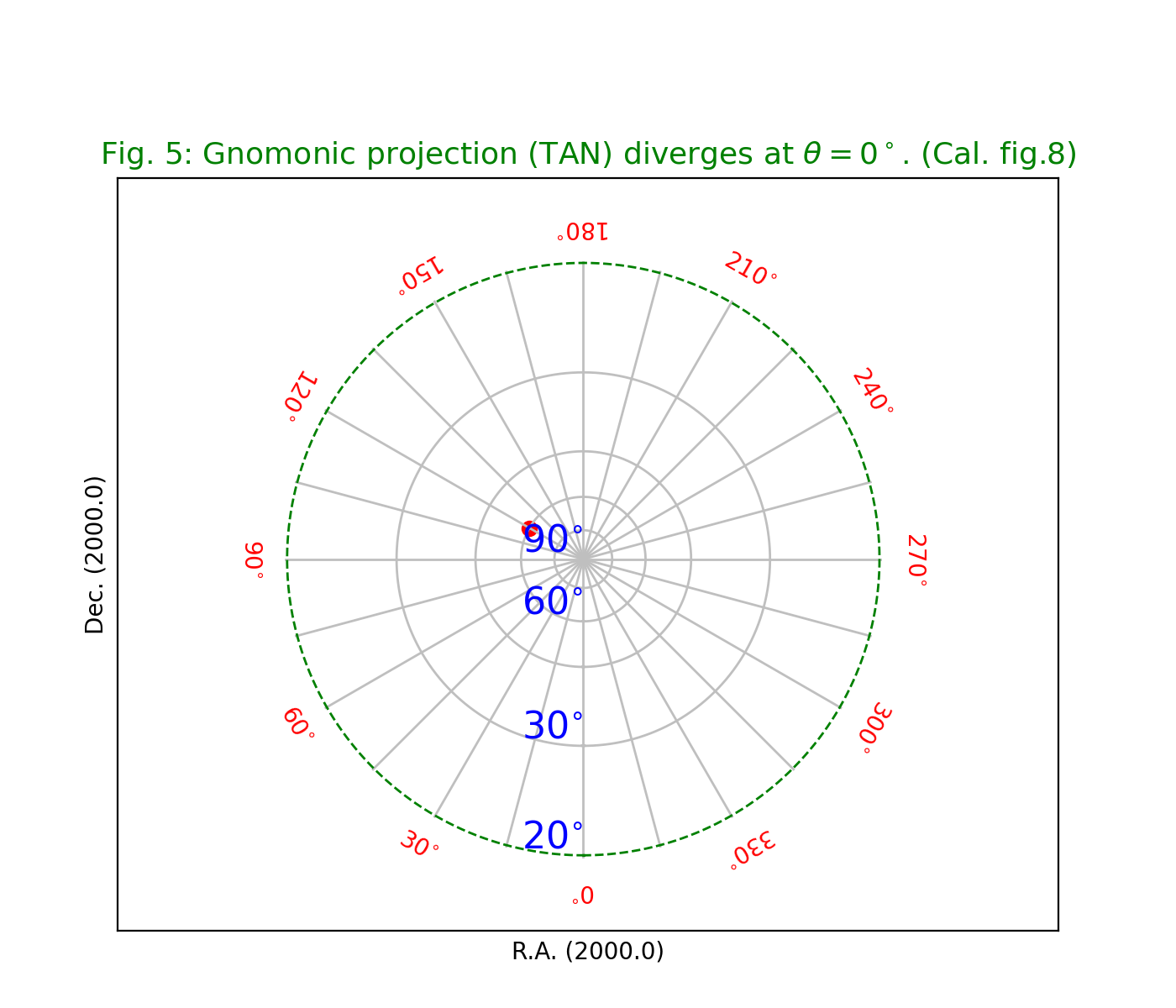
Fig.5: Gnomonic projection (TAN)
In a Gnomonic projection all great circles are
projected as straight lines.
This is nice example of a projection which diverges at certain latitude.
We chose to draw the last border at 20 deg. and plotted it with dashes
using method wcsgrat.Graticule.setp_lineswcs1() as in
grat.setp_lineswcs1(20, color='g', linestyle='--') and identified
the graticule line with its position i.e. latitude 20 deg.
from kapteyn import maputils
import numpy
from service import *

fignum = 5
fig = plt.figure(figsize=figsize)
frame = fig.add_axes(plotbox)
title = r"Gnomonic projection (TAN) diverges at $\theta=0^\circ$. (Cal. fig.8)"
header = {'NAXIS' : 2, 'NAXIS1': 100, 'NAXIS2': 80,
          'CTYPE1' : 'RA---TAN',
          'CRVAL1' :0.0, 'CRPIX1' : 50, 'CUNIT1' : 'deg', 'CDELT1' : -5.0,
          'CTYPE2' : 'DEC--TAN',
          'CRVAL2' : dec0, 'CRPIX2' : 40, 'CUNIT2' : 'deg', 'CDELT2' : 5.0,
         }
X = numpy.arange(0,360.0,15.0)
Y = [20, 30,45, 60, 75]
f = maputils.FITSimage(externalheader=header)
annim = f.Annotatedimage(frame)
grat = annim.Graticule(axnum= (1,2),
                       wylim=(20.0,90.0), wxlim=(0,360),
                       startx=X, starty=Y)
lat_constval = 18
lon_world = list(range(0,360,30))
lat_world = [20, 30, 60, dec0]
labkwargs0 = {'color':'r', 'va':'center', 'ha':'center'}
labkwargs1 = {'color':'b', 'va':'bottom', 'ha':'right', 'fontsize':16}
grat.setp_lineswcs1(20, color='g', linestyle='--')
addangle0 = -90
doplot(frame, fignum, annim, grat, title,
       lon_world=lon_world, lat_world=lat_world, lat_constval=lat_constval,
       addangle0=addangle0, labkwargs0=labkwargs0, labkwargs1=labkwargs1,
       markerpos=markerpos)
(Source code, png, hires.png, pdf)
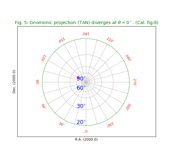
Fig.6: Stereographic projection (STG)
from kapteyn import maputils
import numpy
from service import *

fignum = 6
fig = plt.figure(figsize=figsize)
frame = fig.add_axes(plotbox)
title = r"Stereographic projection (STG) diverges at $\theta=-90^\circ$. (Cal. fig.9)"
header = {'NAXIS' : 2, 'NAXIS1': 100, 'NAXIS2': 80,
          'CTYPE1' : 'RA---STG',
          'CRVAL1' :0.0, 'CRPIX1' : 50, 'CUNIT1' : 'deg', 'CDELT1' : -12.0,
          'CTYPE2' : 'DEC--STG',
          'CRVAL2' : dec0, 'CRPIX2' : 40, 'CUNIT2' : 'deg', 'CDELT2' : 12.0,
         }
X = numpy.arange(0,360.0,30.0)
Y = numpy.arange(-60,90,10.0)
f = maputils.FITSimage(externalheader=header)
annim = f.Annotatedimage(frame)
grat = annim.Graticule(axnum= (1,2),
                       wylim=(-60,90.0), wxlim=(0,360),
                       startx=X, starty=Y)
lat_constval = -62
lon_world = list(range(0,360,30))
lat_world = list(range(-50, 10, 10))
addangle0 = -90
labkwargs1 = {'color':'b', 'va':'bottom', 'ha':'right'}
doplot(frame, fignum, annim, grat, title,
       lon_world=lon_world, lat_world=lat_world, lat_constval=lat_constval,
       addangle0=addangle0, labkwargs1=labkwargs1, markerpos=markerpos)
(Source code, png, hires.png, pdf)

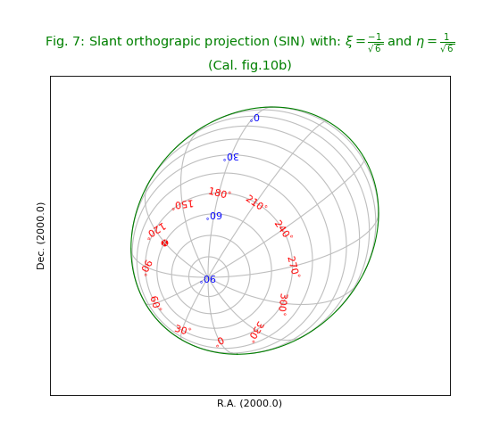
Fig.7: Slant orthographic projection (SIN)
The green colored border is calculated with a border formula given in [Ref2]
from kapteyn import maputils
import numpy
from service import *

fignum = 7
fig = plt.figure(figsize=figsize)
frame = fig.add_axes(plotbox)
t1 = r"""Slant orthograpic projection (SIN) with: """
t2 = r"""$\xi=\frac{-1}{\sqrt{6}}$ and $\eta=\frac{1}{\sqrt{6}}$
(Cal. fig.10b)"""
title = t1 + t2
xi =  -1/numpy.sqrt(6); eta = 1/numpy.sqrt(6)
header = {'NAXIS' : 2, 'NAXIS1': 100, 'NAXIS2': 80,
          'CTYPE1' : 'RA---SIN',
          'CRVAL1' :0.0, 'CRPIX1' : 40, 'CUNIT1' : 'deg', 'CDELT1' : -2,
          'CTYPE2' : 'DEC--SIN',
          'CRVAL2' : dec0, 'CRPIX2' : 30, 'CUNIT2' : 'deg', 'CDELT2' : 2,
          'PV2_1'  : xi, 'PV2_2'  : eta
         }
X = numpy.arange(0,360.0,30.0)
Y = numpy.arange(-90,90,10.0)
f = maputils.FITSimage(externalheader=header)
annim = f.Annotatedimage(frame)
grat = annim.Graticule(axnum= (1,2),
                       wylim=(-90,90.0), wxlim=(0,360),
                       startx=X, starty=Y)
# Special care for the boundary (algorithm from Calabretta et al)
a = numpy.linspace(0,360,500)
arad = a*numpy.pi/180.0
thetaxrad = -numpy.arctan(xi*numpy.sin(arad)-eta*numpy.cos(arad))
thetax = thetaxrad * 180.0/numpy.pi + 0.000001  # Little shift to avoid NaN's at border
g = grat.addgratline(a, thetax, pixels=False)
grat.setp_linespecial(g, color='g', lw=1)
lat_constval = 50
lon_constval = 180
lat_world = [0,30,60,dec0]
lon_world = list(range(0,360,30))
addangle0 = -90
addangle1 = -180
doplot(frame, fignum, annim, grat, title,
       lon_world=lon_world, lat_world=lat_world,
       lon_constval=lon_constval, lat_constval=lat_constval,
       addangle0=addangle0, addangle1=addangle1, markerpos=markerpos)
(Source code, png, hires.png, pdf)

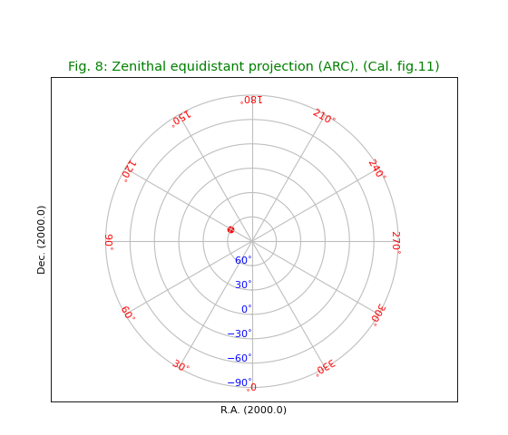
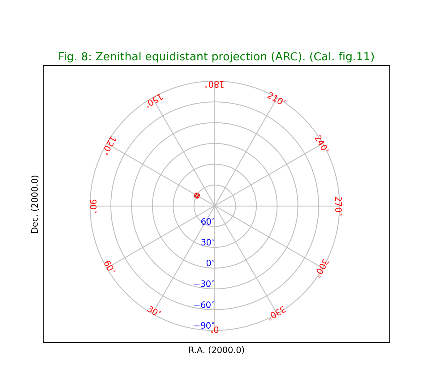
Fig.8: Zenithal equidistant projection (ARC)
from kapteyn import maputils
import numpy
from service import *

fignum = 8
fig = plt.figure(figsize=figsize)
frame = fig.add_axes(plotbox)
title = r"Zenithal equidistant projection (ARC). (Cal. fig.11)"
header = {'NAXIS' : 2, 'NAXIS1': 100, 'NAXIS2': 80,
          'CTYPE1' : 'RA---ARC',
          'CRVAL1' :0.0, 'CRPIX1' : 50, 'CUNIT1' : 'deg', 'CDELT1' : -5.0,
          'CTYPE2' : 'DEC--ARC',
          'CRVAL2' : dec0, 'CRPIX2' : 40, 'CUNIT2' : 'deg', 'CDELT2' : 5.0
         }
X = numpy.arange(0,360.0,30.0)
Y = numpy.arange(-90,90,30.0)
Y[0]= -89.999999   # Graticule for -90 exactly is not plotted
f = maputils.FITSimage(externalheader=header)
annim = f.Annotatedimage(frame)
grat = annim.Graticule(axnum= (1,2), wylim=(-90,90.0), wxlim=(0,360),
                        startx=X, starty=Y)

addangle0 = -90
lat_constval = -87
labkwargs0 = {'color':'r', 'va':'center', 'ha':'center'}
labkwargs1 = {'color':'b', 'va':'bottom', 'ha':'right'}
doplot(frame, fignum, annim, grat, title,
       lat_constval=lat_constval,
       labkwargs0=labkwargs0, labkwargs1=labkwargs1,
       addangle0=addangle0, markerpos=markerpos)
(Source code, png, hires.png, pdf)

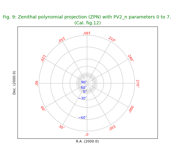
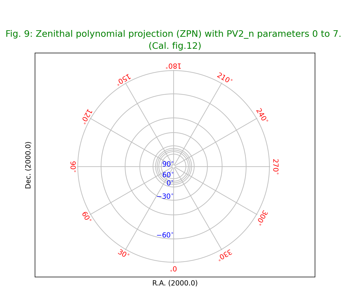
Fig.9: Zenithal polynomial projection (ZPN)
Diverges at some latitude depending on the selected parameters in the PV keywords. Note that the inverse of the polynomial cannot be expressed analytically and there is no function that can transform our marker at \((120^\circ,60^\circ)\) to pixel coordinates.
from kapteyn import maputils
import numpy
from service import *

fignum = 9
fig = plt.figure(figsize=figsize)
frame = fig.add_axes(plotbox)

title = r"""Zenithal polynomial projection (ZPN) with PV2_n parameters 0 to 7.
(Cal. fig.12)"""
header = {'NAXIS' : 2, 'NAXIS1': 100, 'NAXIS2': 80,
         'CTYPE1' : 'RA---ZPN',
         'CRVAL1' :0.0, 'CRPIX1' : 50, 'CUNIT1' : 'deg', 'CDELT1' : -5.0,
         'CTYPE2' : 'DEC--ZPN',
         'CRVAL2' : dec0, 'CRPIX2' : 40, 'CUNIT2' : 'deg', 'CDELT2' : 5.0,
         'PV2_0' : 0.05, 'PV2_1' : 0.975, 'PV2_2' : -0.807,
         'PV2_3' : 0.337, 'PV2_4' : -0.065,
         'PV2_5' : 0.01, 'PV2_6' : 0.003,' PV2_7' : -0.001
         }
X = numpy.arange(0,360.0,30.0)
# Y diverges (this depends on selected parameters). Take save range.
Y = [-70, -60, -45, -30, 0, 15, 30, 45, 60]
f = maputils.FITSimage(externalheader=header)
annim = f.Annotatedimage(frame)
grat = annim.Graticule(axnum= (1,2), wylim=(-70,90.0), wxlim=(0,360),
                      startx=X, starty=Y)
# Configure annotations
lat_constval = -72
lat_world = [-60, -30, 0, 60, dec0]
addangle0 = -90
labkwargs0 = {'color':'r', 'va':'center', 'ha':'center'}
labkwargs1 = {'color':'b', 'va':'bottom', 'ha':'right'}
# No marker position because this can not be evaluated for this projection
# (which has no inverse),
doplot(frame, fignum, annim, grat, title,
       lat_world=lat_world,
       labkwargs0=labkwargs0, labkwargs1=labkwargs1,
       lat_constval=lat_constval, addangle0=addangle0)
(Source code, png, hires.png, pdf)

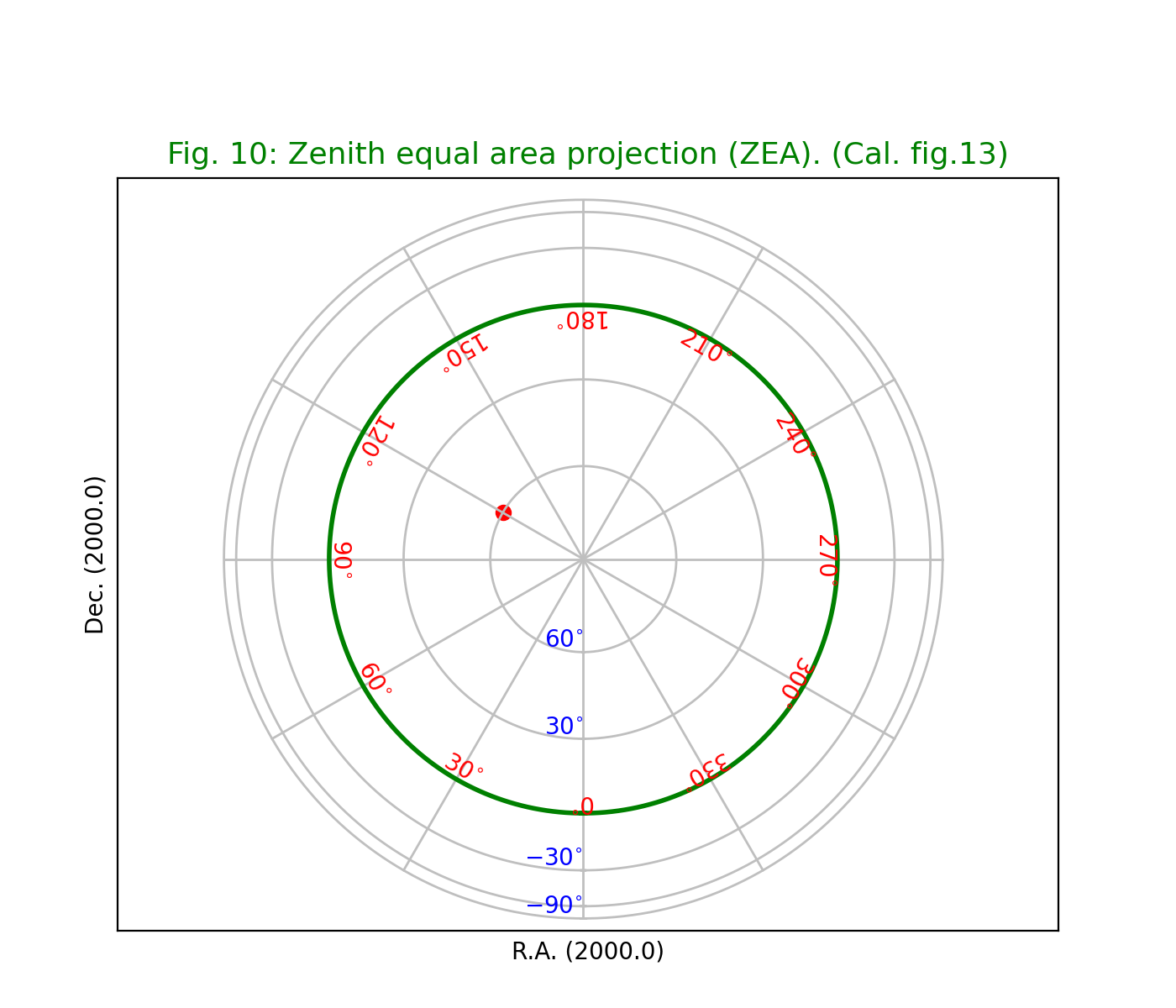
Fig.10: Zenith equal area projection (ZEA)
from kapteyn import maputils
import numpy
from service import *

fignum = 10
fig = plt.figure(figsize=figsize)
frame = fig.add_axes(plotbox)
title = r"Zenith equal area projection (ZEA). (Cal. fig.13)"
header = {'NAXIS' : 2, 'NAXIS1': 100, 'NAXIS2': 80,
          'CTYPE1' : 'RA---ZEA',
          'CRVAL1' :0.0, 'CRPIX1' : 50, 'CUNIT1' : 'deg', 'CDELT1' : -3.0,
          'CTYPE2' : 'DEC--ZEA',
          'CRVAL2' : dec0, 'CRPIX2' : 40, 'CUNIT2' : 'deg', 'CDELT2' : 3.0
         }
X = numpy.arange(0,360.0,30.0)
Y = numpy.arange(-90,90,30.0)
Y[0]= -dec0+0.00000001
f = maputils.FITSimage(externalheader=header)
annim = f.Annotatedimage(frame)
grat = annim.Graticule(axnum= (1,2), wylim=(-90,90.0), wxlim=(0,360),
                       startx=X, starty=Y)
# Set attributes for graticule line at lat = 0
grat.setp_lineswcs1(position=0, color='g', lw=2)
lat_world = [-dec0, -30, 30, 60]
addangle0 = -90
lat_constval = 5.0
labkwargs0 = {'color':'r', 'va':'center', 'ha':'center'}
labkwargs1 = {'color':'b', 'va':'bottom', 'ha':'right'}
doplot(frame, fignum, annim, grat, title,
       lat_world=lat_world,  lat_constval=lat_constval,
       labkwargs0=labkwargs0, labkwargs1=labkwargs1,
       addangle0=addangle0, markerpos=markerpos)
(Source code, png, hires.png, pdf)
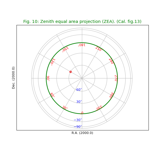
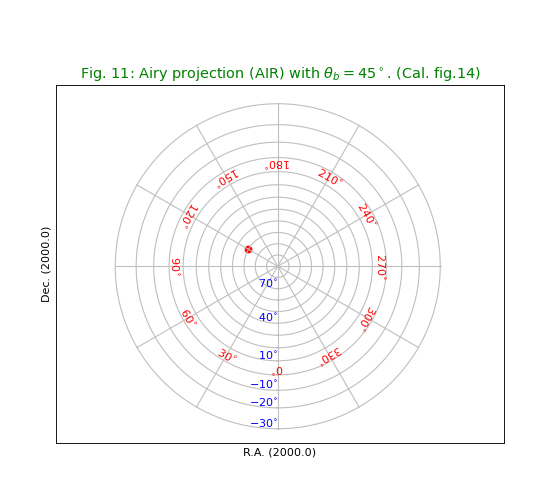
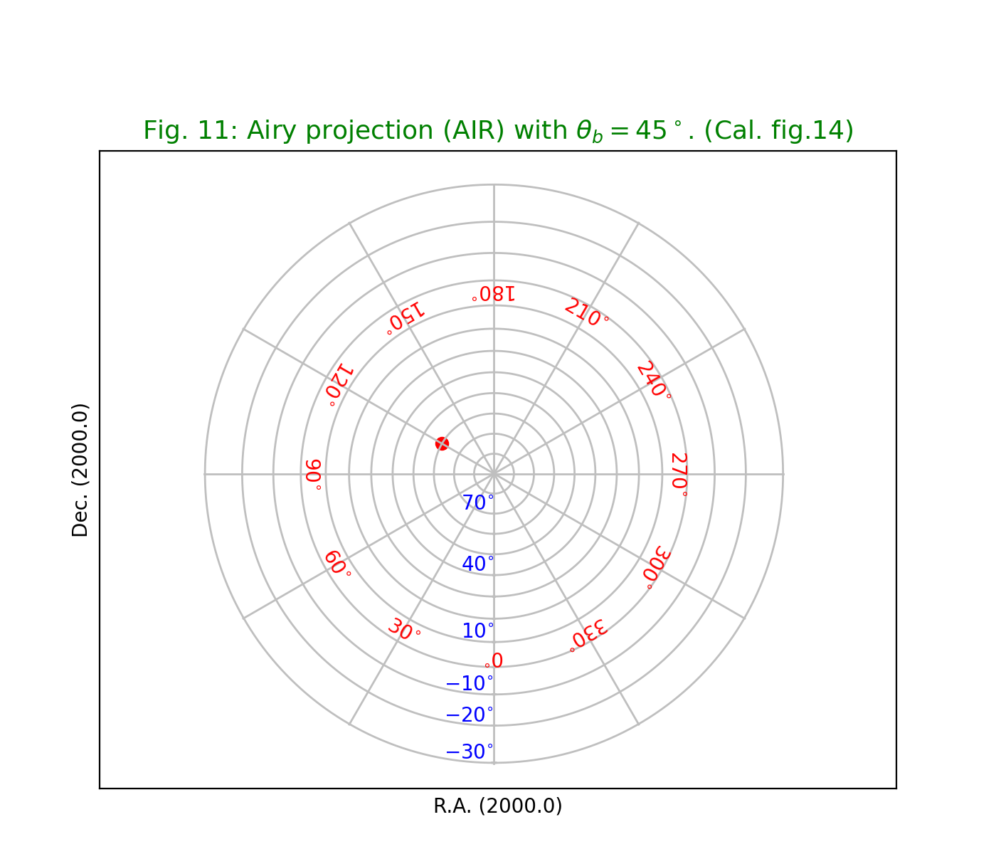
Fig.11: Airy projection (AIR)
from kapteyn import maputils
import numpy
from service import *

fignum = 11
fig = plt.figure(figsize=figsize)
frame = fig.add_axes(plotbox)
title = r"Airy projection (AIR) with $\theta_b = 45^\circ$. (Cal. fig.14)"
header = {'NAXIS' : 2, 'NAXIS1': 100, 'NAXIS2': 80,
          'CTYPE1' : 'RA---AIR',
          'CRVAL1' :0.0, 'CRPIX1' : 50, 'CUNIT1' : 'deg', 'CDELT1' : -4.0,
          'CTYPE2' : 'DEC--AIR',
          'CRVAL2' : dec0, 'CRPIX2' : 40, 'CUNIT2' : 'deg', 'CDELT2' : 4.0
         }
X = numpy.arange(0,360.0,30.0)
Y = numpy.arange(-30,90,10.0)
# Diverges at dec = -90, start at dec = -30
f = maputils.FITSimage(externalheader=header)
annim = f.Annotatedimage(frame)
grat = annim.Graticule(axnum= (1,2), wylim=(-30,90.0), wxlim=(0,360),
                        startx=X, starty=Y)
lat_world = [-30, -20, -10, 10, 40, 70]
addangle0 = -90
lat_constval = 4.0
labkwargs0 = {'color':'r', 'va':'center', 'ha':'center'}
labkwargs1 = {'color':'b', 'va':'bottom', 'ha':'right'}
doplot(frame, fignum, annim, grat, title,
       lat_world=lat_world, lat_constval=lat_constval,
       labkwargs0=labkwargs0, labkwargs1=labkwargs1,
       addangle0=addangle0, markerpos=markerpos)
(Source code, png, hires.png, pdf)

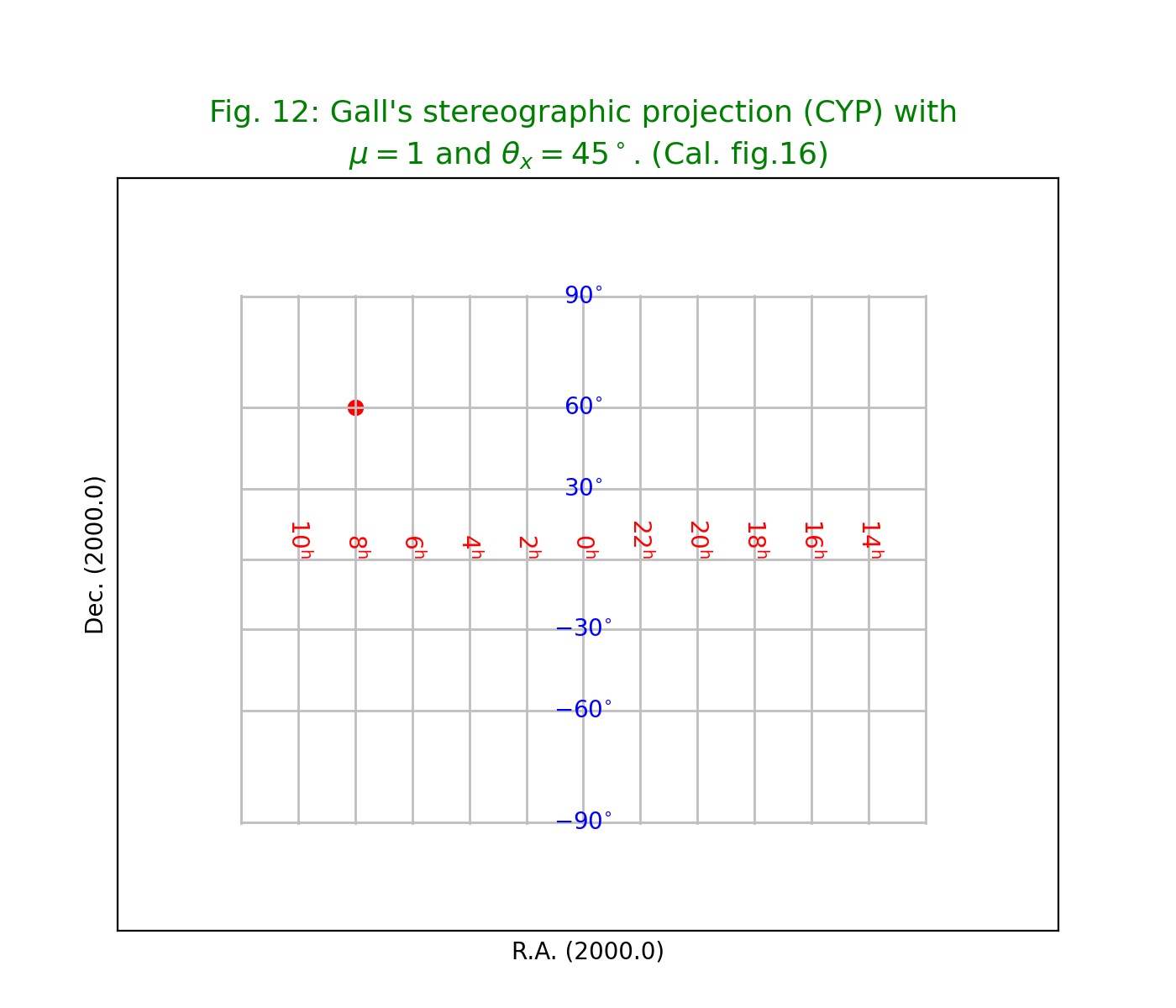
Cylindrical Projections
The native coordinate system origin of a Cylindrical projection coincides with the reference point. Therefore we set \((\phi_0, \theta_0) = (0,0)\)
Fig.12: Gall’s stereographic projection (CYP)
from kapteyn import maputils
import numpy
from service import *

fignum = 12
fig = plt.figure(figsize=figsize)
frame = fig.add_axes(plotbox)
title =  r"""Gall's stereographic projection (CYP) with
$\mu = 1$ and $\theta_x = 45^\circ$. (Cal. fig.16)"""
header = {'NAXIS'  : 2, 'NAXIS1': 100, 'NAXIS2': 80,
          'CTYPE1' : 'RA---CYP',
          'CRVAL1' : 0.0, 'CRPIX1' : 50, 'CUNIT1' : 'deg', 'CDELT1' : -3.5,
          'CTYPE2' : 'DEC--CYP',
          'CRVAL2' : 0.0, 'CRPIX2' : 40, 'CUNIT2' : 'deg', 'CDELT2' : 3.5,
          'PV2_1'  : 1, 'PV2_2' : numpy.sqrt(2.0)/2.0
         }
X = cylrange()
Y = numpy.arange(-90,100,30.0)  # i.e. include +90 also
f = maputils.FITSimage(externalheader=header)
annim = f.Annotatedimage(frame)
grat = annim.Graticule(axnum= (1,2), wylim=(-90,90.0), wxlim=(0,360),
                       startx=X, starty=Y)
lat_world = [-90, -60,-30, 30, 60, dec0]
# Trick to get the right longs.
w1 = numpy.arange(0,179,30.0)
w2 = numpy.arange(210,360,30.0)
lon_world = numpy.concatenate((w1, w2))
labkwargs0 = {'color':'r', 'va':'bottom', 'ha':'center'}
labkwargs1 = {'color':'b', 'va':'center', 'ha':'center'}
doplot(frame, fignum, annim, grat, title,
       lon_world=lon_world, lat_world=lat_world,
       labkwargs0=labkwargs0, labkwargs1=labkwargs1,
       lon_fmt='Hms', markerpos=markerpos)
(Source code, png, hires.png, pdf)
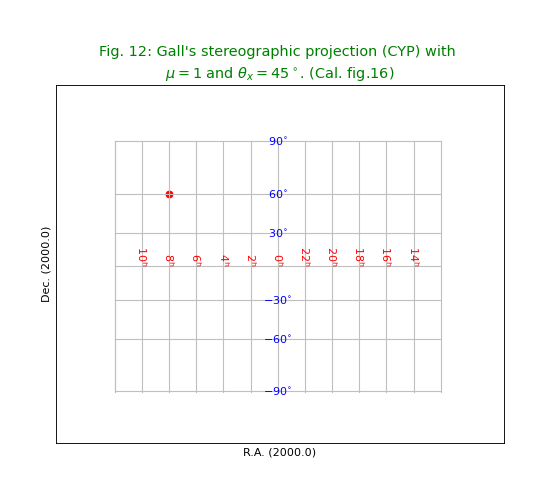
Fig.13: Lambert’s equal area projection (CEA)
from kapteyn import maputils
import numpy
from service import *

fignum = 13
fig = plt.figure(figsize=figsize)
frame = fig.add_axes(plotbox)
title = r"Lambert's equal area projection (CEA) with $\lambda = 1$. (Cal. fig.17)"
header = {'NAXIS'  : 2, 'NAXIS1': 100, 'NAXIS2': 80,
          'CTYPE1' : 'RA---CEA',
          'CRVAL1' : 0.0, 'CRPIX1' : 50, 'CUNIT1' : 'deg', 'CDELT1' : -5.0,
          'CTYPE2' : 'DEC--CEA',
          'CRVAL2' : 0.0, 'CRPIX2' : 40, 'CUNIT2' : 'deg', 'CDELT2' : 5.0,
          'PV2_1'  : 1
         }
X = cylrange()
Y = numpy.arange(-90,100,30.0)  # i.e. include +90 also
f = maputils.FITSimage(externalheader=header)
annim = f.Annotatedimage(frame)
grat = annim.Graticule(axnum= (1,2), wylim=(-90,90.0), wxlim=(0,360),
                       startx=X, starty=Y)
lat_world = [-60,-30, 30, 60]
#lon_world = range(0,360,30)
#lon_world.append(180+epsilon)
w1 = numpy.arange(0,179,30.0)
w2 = numpy.arange(180,360,30.0)
w2[0] = 180 + epsilon
lon_world = numpy.concatenate((w1, w2))
labkwargs0 = {'color':'r', 'va':'bottom', 'ha':'right'}
labkwargs1 = {'color':'b', 'va':'center', 'ha':'right'}
doplot(frame, fignum, annim, grat, title,
       lon_world=lon_world, lat_world=lat_world,
       labkwargs0=labkwargs0, labkwargs1=labkwargs1,
       deltapy1=0.5,
       markerpos=markerpos)
(Source code, png, hires.png, pdf)

Fig.14: Plate Carree projection (CAR)
from kapteyn import maputils
import numpy
from service import *

fignum = 14
fig = plt.figure(figsize=figsize)
frame = fig.add_axes(plotbox)
title = "Plate Carree projection (CAR). (Cal. fig.18)"
header = {'NAXIS'  : 2, 'NAXIS1': 100, 'NAXIS2': 80,
          'CTYPE1' : 'RA---CAR',
          'CRVAL1' : 0.0, 'CRPIX1' : 50, 'CUNIT1' : 'deg', 'CDELT1' : -4.0,
          'CTYPE2' : 'DEC--CAR',
          'CRVAL2' : 0.0, 'CRPIX2' : 40, 'CUNIT2' : 'deg', 'CDELT2' : 4.0,
         }
X = cylrange()
Y = numpy.arange(-90,100,30.0)  # i.e. include +90 also
f = maputils.FITSimage(externalheader=header)
annim = f.Annotatedimage(frame)
grat = annim.Graticule(axnum= (1,2), wylim=(-90,90.0), wxlim=(0,360),
                        startx=X, starty=Y)
lat_world = [-90, -60,-30, 0, 30, 60, dec0]
# Remove the left 180 deg and print the right 180 deg instead
w1 = numpy.arange(0,179,30.0)
w2 = numpy.arange(180,360,30.0)
w2[0] = 180 + epsilon
lon_world = numpy.concatenate((w1, w2))
labkwargs0 = {'color':'r', 'va':'top', 'ha':'right'}
labkwargs1 = {'color':'b', 'va':'bottom', 'ha':'right'}
doplot(frame, fignum, annim, grat, title,
       lon_world=lon_world, lat_world=lat_world,
       labkwargs0=labkwargs0, labkwargs1=labkwargs1,
       markerpos=markerpos)
(Source code, png, hires.png, pdf)
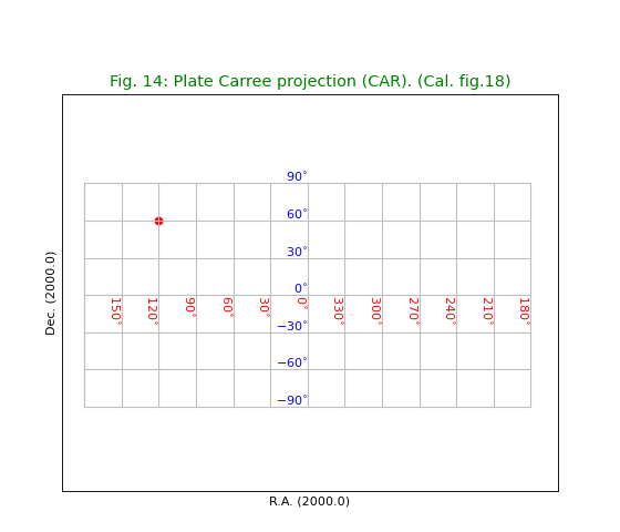
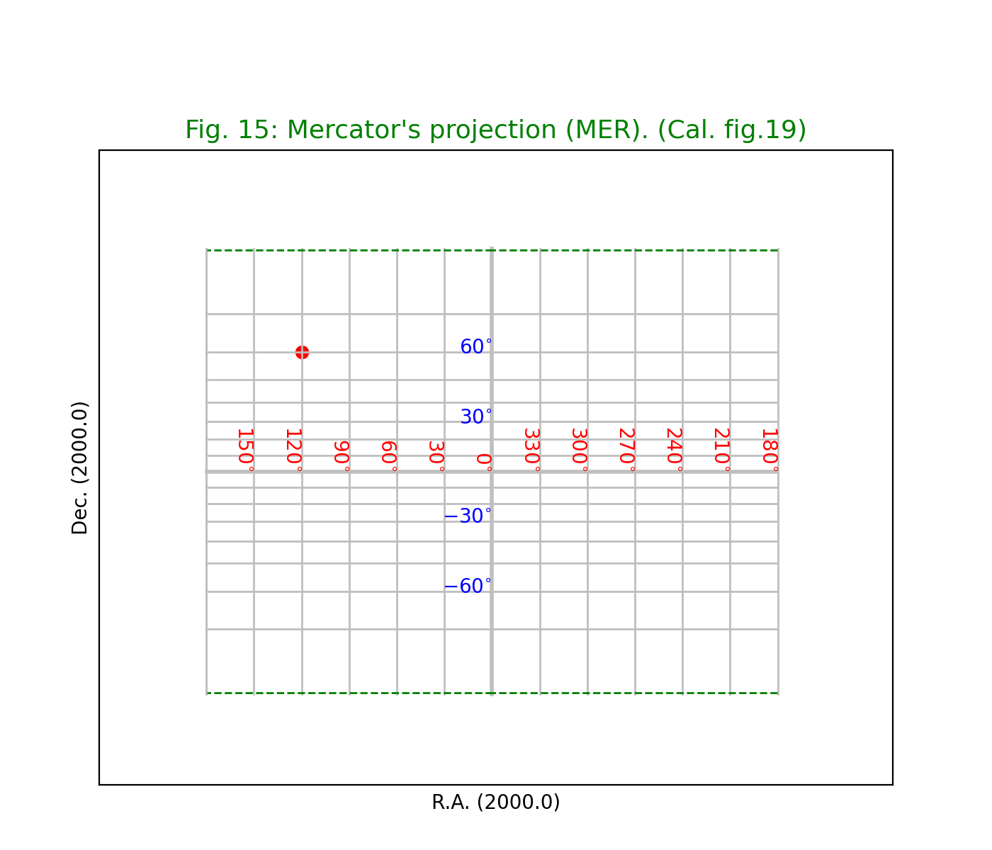
Fig.15: Mercator’s projection (MER)
from kapteyn import maputils
import numpy
from service import *

fignum = 15
fig = plt.figure(figsize=figsize)
frame = fig.add_axes(plotbox)
title =  "Mercator's projection (MER). (Cal. fig.19)"
header = {'NAXIS'  : 2, 'NAXIS1': 100, 'NAXIS2': 80,
          'CTYPE1' : 'RA---MER',
          'CRVAL1' : 0.0, 'CRPIX1' : 50, 'CUNIT1' : 'deg', 'CDELT1' : -5.0,
          'CTYPE2' : 'DEC--MER',
          'CRVAL2' : 0.0, 'CRPIX2' : 40, 'CUNIT2' : 'deg', 'CDELT2' : 5.0,
         }
X = cylrange()
Y = numpy.arange(-80,90,10.0)  # Diverges at +-90 so exclude these values
f = maputils.FITSimage(externalheader=header)
annim = f.Annotatedimage(frame)
grat = annim.Graticule(header, axnum= (1,2), wylim=(-80,80.0), wxlim=(0,360),
                       startx=X, starty=Y)
grat.setp_lineswcs1((-80,80), linestyle='--', color='g')
grat.setp_lineswcs0(0, lw=2)
grat.setp_lineswcs1(0, lw=2)
lat_world = [-60,-30, 30, 60]
# Remove the left 180 deg and print the right 180 deg instead
w1 = numpy.arange(0,179,30.0)
w2 = numpy.arange(180,360,30.0)
w2[0] = 180 + epsilon
lon_world = numpy.concatenate((w1, w2))
labkwargs0 = {'color':'r', 'va':'bottom', 'ha':'right'}
labkwargs1 = {'color':'b', 'va':'center', 'ha':'right'}
doplot(frame, fignum, annim, grat, title,
       lon_world=lon_world, lat_world=lat_world,
       deltapy1=0.5,
       labkwargs0=labkwargs0, labkwargs1=labkwargs1,
       markerpos=markerpos)
(Source code, png, hires.png, pdf)

Pseudocylindrical projections
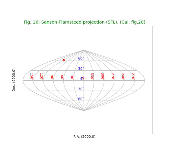
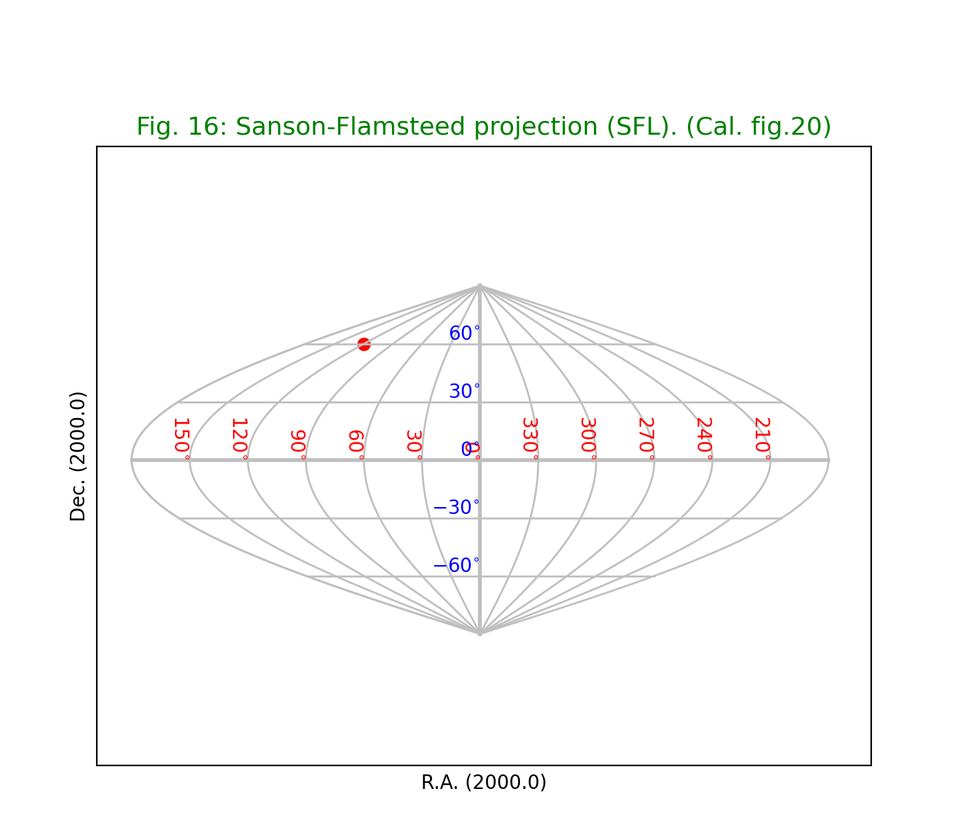
Fig.16: Sanson-Flamsteed projection (SFL)
from kapteyn import maputils
import numpy
from service import *

fignum = 16
fig = plt.figure(figsize=figsize)
frame = fig.add_axes(plotbox)
title = "Sanson-Flamsteed projection (SFL). (Cal. fig.20)"
header = {'NAXIS'  : 2, 'NAXIS1': 100, 'NAXIS2': 80,
            'CTYPE1' : 'RA---SFL',
            'CRVAL1' : 0.0, 'CRPIX1' : 50, 'CUNIT1' : 'deg', 'CDELT1' : -4.0,
            'CTYPE2' : 'DEC--SFL',
            'CRVAL2' : 0.0, 'CRPIX2' : 40, 'CUNIT2' : 'deg', 'CDELT2' : 4.0,
         }
X = cylrange()
Y = numpy.arange(-60,90,30.0)
f = maputils.FITSimage(externalheader=header)
annim = f.Annotatedimage(frame)
grat = annim.Graticule(axnum= (1,2), wylim=(-90,90.0), wxlim=(0,360),
                       startx=X, starty=Y)
grat.setp_lineswcs0(0, lw=2)
grat.setp_lineswcs1(0, lw=2)
lat_world = [-60,-30, 0, 30, 60]
# Remove the left 180 deg and print the right 180 deg instead
w1 = numpy.arange(0,151,30.0)
w2 = numpy.arange(210,360,30.0)
lon_world = numpy.concatenate((w1, w2))
labkwargs0 = {'color':'r', 'va':'bottom', 'ha':'right'}
labkwargs1 = {'color':'b', 'va':'bottom', 'ha':'right'}
doplot(frame, fignum, annim, grat, title,
       lon_world=lon_world, lat_world=lat_world,
       labkwargs0=labkwargs0, labkwargs1=labkwargs1,
       markerpos=markerpos)
(Source code, png, hires.png, pdf)

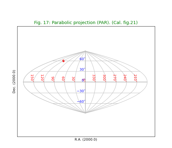
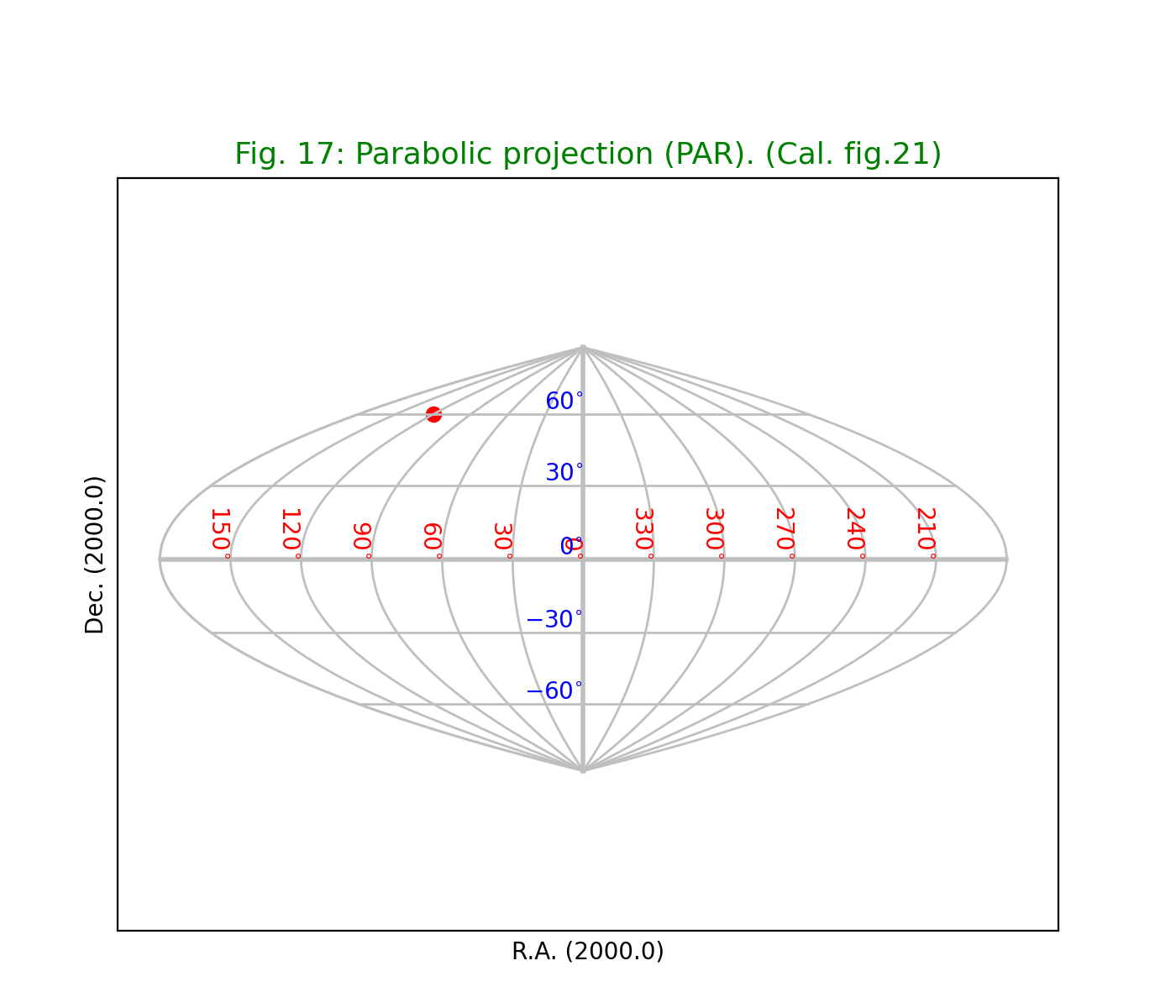
Fig.17: Parabolic projection (PAR)
from kapteyn import maputils
import numpy
from service import *

fignum = 17
fig = plt.figure(figsize=figsize)
frame = fig.add_axes(plotbox)
title = "Parabolic projection (PAR). (Cal. fig.21)"
header = {'NAXIS'  : 2, 'NAXIS1': 100, 'NAXIS2': 80,
          'CTYPE1' : 'RA---PAR',
          'CRVAL1' : 0.0, 'CRPIX1' : 50, 'CUNIT1' : 'deg', 'CDELT1' : -4.0,
          'CTYPE2' : 'DEC--PAR',
          'CRVAL2' : 0.0, 'CRPIX2' : 40, 'CUNIT2' : 'deg', 'CDELT2' : 4.0,
         }
X = cylrange()
Y = numpy.arange(-60,90,30.0)
f = maputils.FITSimage(externalheader=header)
annim = f.Annotatedimage(frame)
grat = annim.Graticule(axnum= (1,2), wylim=(-90,90.0), wxlim=(0,360),
                       startx=X, starty=Y)
grat.setp_lineswcs0(0, lw=2)
grat.setp_lineswcs1(0, lw=2)
lat_world = [-60,-30, 0, 30, 60]
# Remove the left 180 deg and print the right 180 deg instead
w1 = numpy.arange(0,151,30.0)
w2 = numpy.arange(210,360,30.0)
lon_world = numpy.concatenate((w1, w2))
labkwargs0 = {'color':'r', 'va':'bottom', 'ha':'right'}
labkwargs1 = {'color':'b', 'va':'bottom', 'ha':'right'}
doplot(frame, fignum, annim, grat, title,
       lon_world=lon_world, lat_world=lat_world,
       lat_constval = 0.0,
       labkwargs0=labkwargs0, labkwargs1=labkwargs1,
       markerpos=markerpos)
(Source code, png, hires.png, pdf)

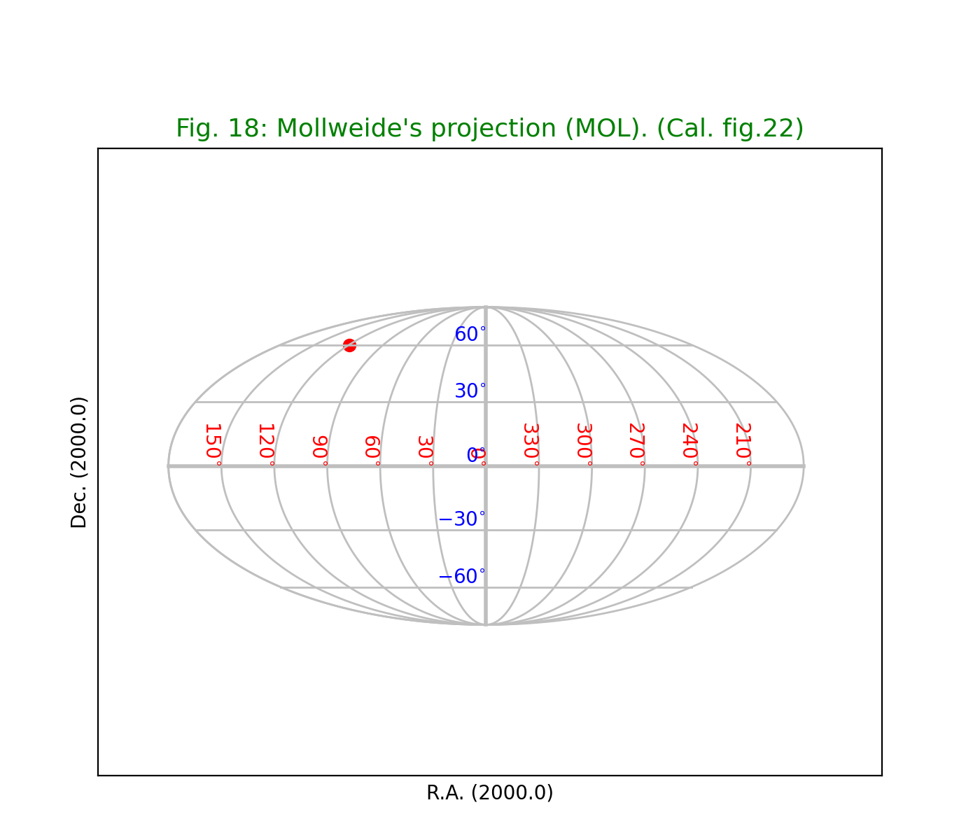
Fig.18: Mollweide’s projection (MOL)
from kapteyn import maputils
import numpy
from service import *

fignum = 18
fig = plt.figure(figsize=figsize)
frame = fig.add_axes(plotbox)
title=  "Mollweide's projection (MOL). (Cal. fig.22)"
header = {'NAXIS'  : 2, 'NAXIS1': 100, 'NAXIS2': 80,
          'CTYPE1' : 'RA---MOL',
          'CRVAL1' : 0.0, 'CRPIX1' : 50, 'CUNIT1' : 'deg', 'CDELT1' : -4.0,
          'CTYPE2' : 'DEC--MOL',
          'CRVAL2' : 0.0, 'CRPIX2' : 40, 'CUNIT2' : 'deg', 'CDELT2' : 4.0,
         }
X = cylrange()
Y = numpy.arange(-60,90,30.0)  # Diverges at +-90 so exclude these values
f = maputils.FITSimage(externalheader=header)
annim = f.Annotatedimage(frame)
grat = annim.Graticule(axnum= (1,2), wylim=(-90,90.0), wxlim=(0,360),
                       startx=X, starty=Y)
grat.setp_lineswcs0(0, lw=2)
grat.setp_lineswcs1(0, lw=2)
lat_world = [-60,-30, 0, 30, 60]
# Remove the left 180 deg and print the right 180 deg instead
w1 = numpy.arange(0,151,30.0)
w2 = numpy.arange(210,360,30.0)
lon_world = numpy.concatenate((w1, w2))
labkwargs0 = {'color':'r', 'va':'bottom', 'ha':'right'}
labkwargs1 = {'color':'b', 'va':'bottom', 'ha':'right'}
doplot(frame, fignum, annim, grat, title,
       lon_world=lon_world, lat_world=lat_world,
       labkwargs0=labkwargs0, labkwargs1=labkwargs1,
       markerpos=markerpos)
(Source code, png, hires.png, pdf)
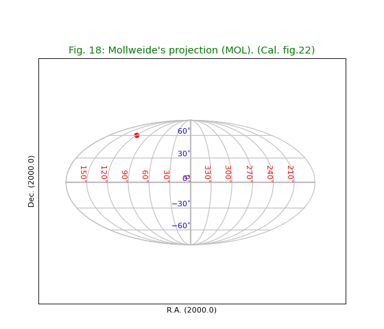
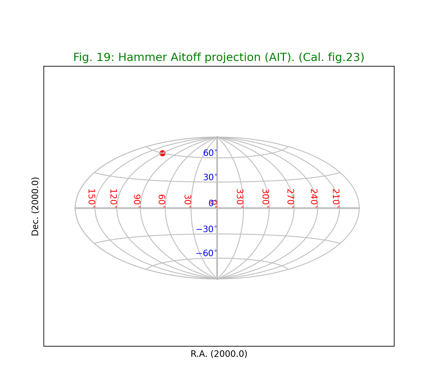
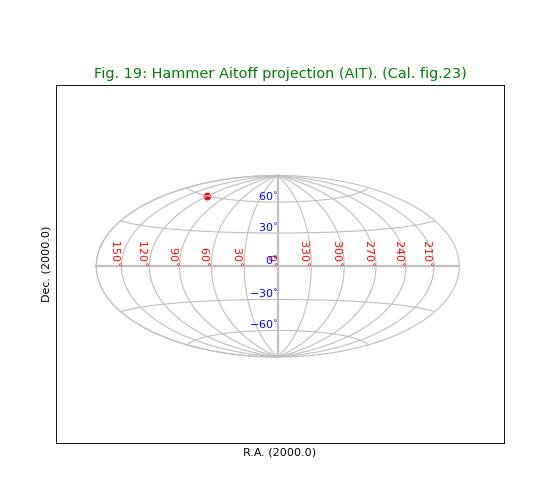
Fig.19: Hammer Aitoff projection (AIT)
from kapteyn import maputils
import numpy
from service import *

fignum = 19
fig = plt.figure(figsize=figsize)
frame = fig.add_axes(plotbox)
title = "Hammer Aitoff projection (AIT). (Cal. fig.23)"
header = {'NAXIS'  : 2, 'NAXIS1': 100, 'NAXIS2': 80,
          'CTYPE1' : 'RA---AIT',
          'CRVAL1' : 0.0, 'CRPIX1' : 50, 'CUNIT1' : 'deg', 'CDELT1' : -4.0,
          'CTYPE2' : 'DEC--AIT',
          'CRVAL2' : 0.0, 'CRPIX2' : 40, 'CUNIT2' : 'deg', 'CDELT2' : 4.0,
         }
X = cylrange()
Y = numpy.arange(-60,90,30.0)
f = maputils.FITSimage(externalheader=header)
annim = f.Annotatedimage(frame)
grat = annim.Graticule(axnum= (1,2), wylim=(-90,90.0), wxlim=(0,360),
                       startx=X, starty=Y)
grat.setp_lineswcs0(0, lw=2)
grat.setp_lineswcs1(0, lw=2)
lat_world = [-60,-30, 0, 30, 60]
# Remove the left 180 deg and print the right 180 deg instead
w1 = numpy.arange(0,151,30.0)
w2 = numpy.arange(210,360,30.0)
lon_world = numpy.concatenate((w1, w2))
labkwargs0 = {'color':'r', 'va':'bottom', 'ha':'right'}
labkwargs1 = {'color':'b', 'va':'bottom', 'ha':'right'}
doplot(frame, fignum, annim, grat, title,
       lon_world=lon_world, lat_world=lat_world,
       labkwargs0=labkwargs0, labkwargs1=labkwargs1,
       markerpos=markerpos)
(Source code, png, hires.png, pdf)
Conic projections
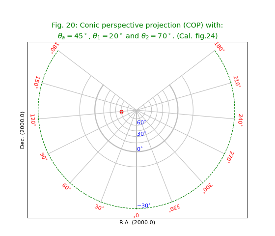
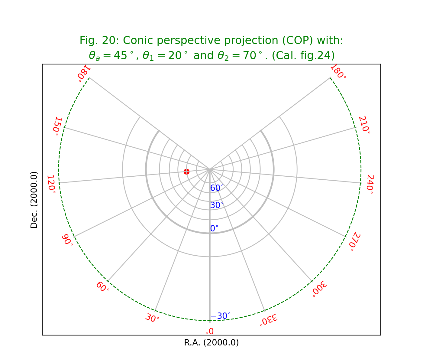
Fig.20: Conic perspective projection (COP)
from kapteyn import maputils
import numpy
from service import *

fignum = 20
fig = plt.figure(figsize=figsize)
frame = fig.add_axes(plotbox)
theta_a = 45
t1 = 20.0; t2 = 70.0
eta = abs(t1-t2)/2.0
title = r"""Conic perspective projection (COP) with:
$\theta_a=45^\circ$, $\theta_1=20^\circ$ and $\theta_2=70^\circ$. (Cal. fig.24)"""
header = {'NAXIS'  : 2, 'NAXIS1': 100, 'NAXIS2': 80,
          'CTYPE1' : 'RA---COP',
          'CRVAL1' : 0.0, 'CRPIX1' : 50, 'CUNIT1' : 'deg', 'CDELT1' : -5.5,
          'CTYPE2' : 'DEC--COP',
          'CRVAL2' : theta_a, 'CRPIX2' : 40, 'CUNIT2' : 'deg', 'CDELT2' : 5.5,
          'PV2_1'  : theta_a, 'PV2_2' : eta
         }
X = numpy.arange(0,370.0,30.0);  X[-1] = 180+epsilon
Y = numpy.arange(-30,90,15.0)  # Diverges at theta_a +- 90.0
f = maputils.FITSimage(externalheader=header)
annim = f.Annotatedimage(frame)
grat = annim.Graticule(axnum= (1,2), wylim=(-30,90.0), wxlim=(0,360),
                       startx=X, starty=Y)
grat.setp_lineswcs1(-30, linestyle='--', color='g')
grat.setp_lineswcs0(0, lw=2)
grat.setp_lineswcs1(0, lw=2)
lon_world = list(range(0,360,30))
lon_world.append(180+epsilon)
lat_world = [-30, 0, 30, 60]
addangle0 = -90
lat_constval = -31
labkwargs0 = {'color':'r', 'va':'center', 'ha':'center'}
labkwargs1 = {'color':'b', 'va':'bottom', 'ha':'left'}
doplot(frame, fignum, annim, grat, title,
       lon_world=lon_world, lat_world=lat_world,
       lat_constval=lat_constval,
       labkwargs0=labkwargs0, labkwargs1=labkwargs1,
       addangle0=addangle0, markerpos=markerpos)
(Source code, png, hires.png, pdf)

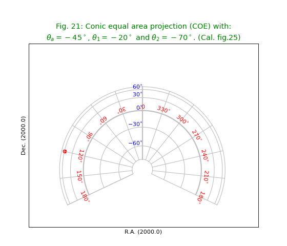
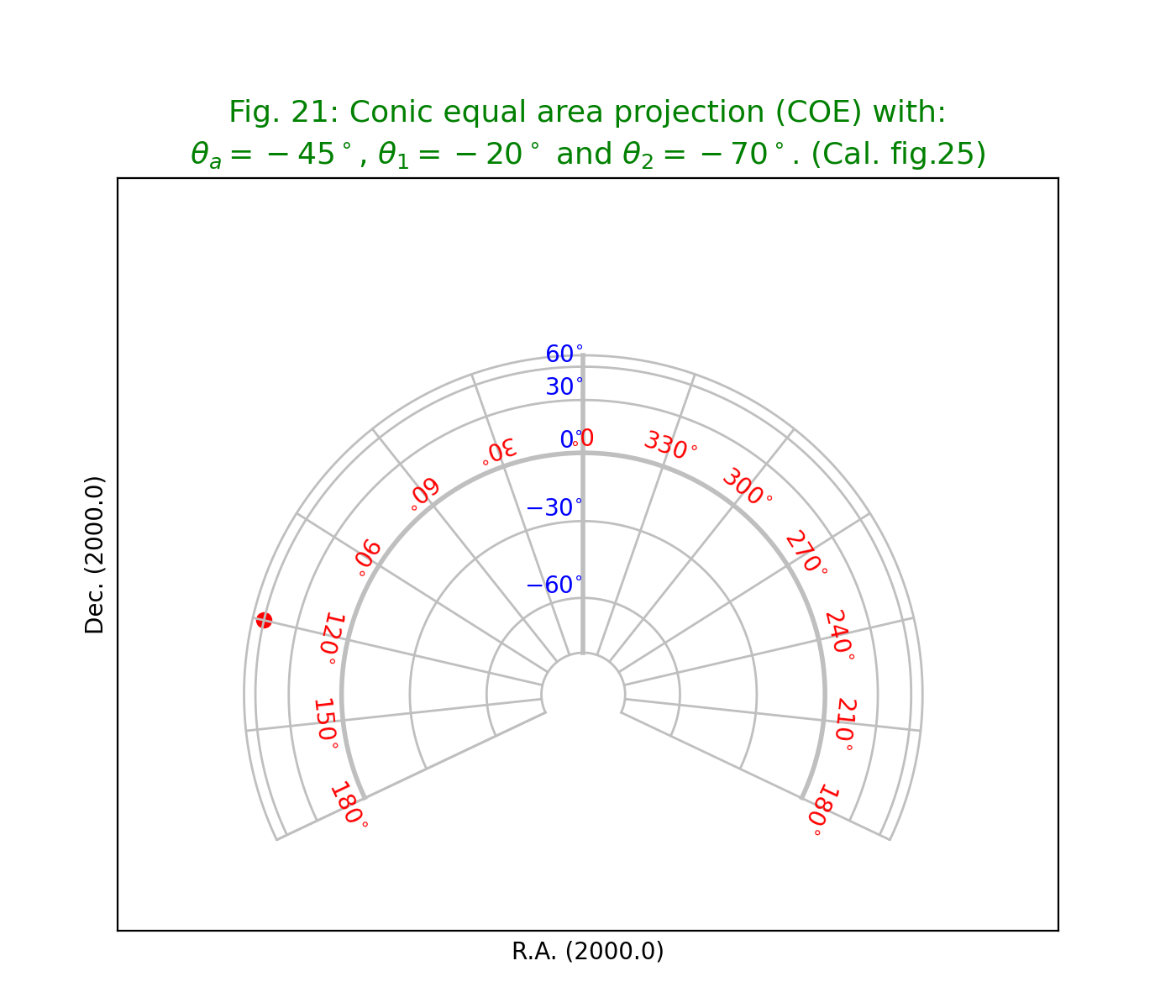
Fig.21: Conic equal area projection (COE)
from kapteyn import maputils
import numpy
from service import *

fignum = 21
fig = plt.figure(figsize=figsize)
frame = fig.add_axes(plotbox)
theta_a = -45
t1 = -20.0; t2 = -70.0
eta = abs(t1-t2)/2.0
title = r"""Conic equal area projection (COE) with:
$\theta_a=-45^\circ$, $\theta_1=-20^\circ$ and $\theta_2=-70^\circ$. (Cal. fig.25)"""
header = {'NAXIS'  : 2, 'NAXIS1': 100, 'NAXIS2': 80,
          'CTYPE1' : 'RA---COE',
          'CRVAL1' : 0.0, 'CRPIX1' : 50, 'CUNIT1' : 'deg', 'CDELT1' : -4.0,
          'CTYPE2' : 'DEC--COE',
          'CRVAL2' : theta_a, 'CRPIX2' : 40, 'CUNIT2' : 'deg', 'CDELT2' : 4.0,
          'PV2_1'  : theta_a, 'PV2_2' : eta
         }
X = cylrange()
Y = numpy.arange(-90,91,30.0); Y[-1] = dec0
f = maputils.FITSimage(externalheader=header)
annim = f.Annotatedimage(frame)
grat = annim.Graticule(axnum= (1,2), wylim=(-90,90.0), wxlim=(0,360),
                       startx=X, starty=Y)
grat.setp_lineswcs0(0, lw=2)
grat.setp_lineswcs1(0, lw=2)
lon_world = list(range(0,360,30))
lon_world.append(180+epsilon)
lat_constval = 10
lat_world = [-60,-30,0,30,60]
addangle0 = -90.0
labkwargs0 = {'color':'r', 'va':'center', 'ha':'center'}
labkwargs1 = {'color':'b', 'va':'bottom', 'ha':'right'}
doplot(frame, fignum, annim, grat, title,
       lon_world=lon_world, lat_world=lat_world,
       lat_constval=lat_constval,
       labkwargs0=labkwargs0, labkwargs1=labkwargs1,
       addangle0=addangle0, markerpos=markerpos)
(Source code, png, hires.png, pdf)

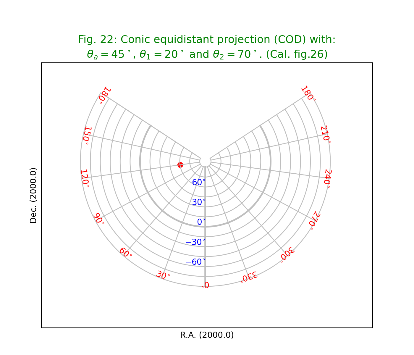
Fig.22: Conic equidistant projection (COD)
from kapteyn import maputils
import numpy
from service import *

fignum = 22
fig = plt.figure(figsize=figsize)
frame = fig.add_axes(plotbox)
theta_a = 45
t1 = 20.0; t2 = 70.0
eta = abs(t1-t2)/2.0
title = r"""Conic equidistant projection (COD) with:
$\theta_a=45^\circ$, $\theta_1=20^\circ$ and $\theta_2=70^\circ$. (Cal. fig.26)"""
header = {'NAXIS'  : 2, 'NAXIS1': 100, 'NAXIS2': 80,
          'CTYPE1' : 'RA---COD',
          'CRVAL1' : 0.0, 'CRPIX1' : 50, 'CUNIT1' : 'deg', 'CDELT1' : -5.0,
          'CTYPE2' : 'DEC--COD',
          'CRVAL2' : theta_a, 'CRPIX2' : 40, 'CUNIT2' : 'deg', 'CDELT2' : 5.0,
          'PV2_1'  : theta_a, 'PV2_2' : eta
         }
X = cylrange()
Y = numpy.arange(-90,91,15)
f = maputils.FITSimage(externalheader=header)
annim = f.Annotatedimage(frame)
grat = annim.Graticule(axnum= (1,2), wylim=(-90,90.0), wxlim=(0,360),
                       startx=X, starty=Y)
grat.setp_lineswcs0(0, lw=2)
grat.setp_lineswcs1(0, lw=2)
lon_world = list(range(0,360,30))
lon_world.append(180.0+epsilon)
addangle0 = -90.0
lat_constval = -86
lat_world = [-60, -30, 0, 30, 60]
labkwargs0 = {'color':'r', 'va':'center', 'ha':'center'}
labkwargs1 = {'color':'b', 'va':'bottom', 'ha':'right'}
doplot(frame, fignum, annim, grat, title,
       lon_world=lon_world, lat_world=lat_world,
       lat_constval=lat_constval,
       labkwargs0=labkwargs0, labkwargs1=labkwargs1,
       addangle0=addangle0, markerpos=markerpos)
(Source code, png, hires.png, pdf)
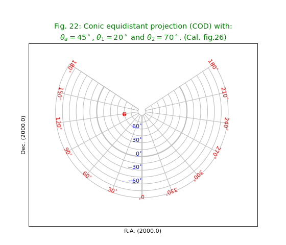
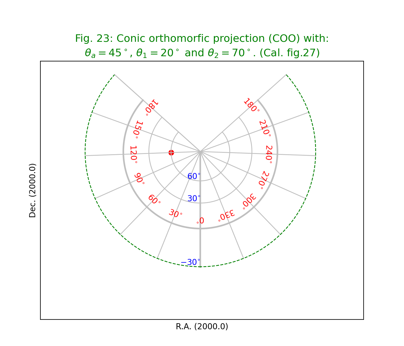
Fig.23: Conic orthomorfic projection (COO)
from kapteyn import maputils
import numpy
from service import *

fignum = 23
fig = plt.figure(figsize=figsize)
frame = fig.add_axes(plotbox)
theta_a = 45
t1 = 20.0; t2 = 70.0
eta = abs(t1-t2)/2.0
title = r"""Conic orthomorfic projection (COO) with:
$\theta_a=45^\circ$, $\theta_1=20^\circ$ and $\theta_2=70^\circ$. (Cal. fig.27)"""
header = {'NAXIS'  : 2, 'NAXIS1': 100, 'NAXIS2': 80,
          'CTYPE1' : 'RA---COO',
          'CRVAL1' : 0.0, 'CRPIX1' : 50, 'CUNIT1' : 'deg', 'CDELT1' : -4.0,
          'CTYPE2' : 'DEC--COO',
          'CRVAL2' : theta_a, 'CRPIX2' : 40, 'CUNIT2' : 'deg', 'CDELT2' : 4.0,
          'PV2_1'  : theta_a, 'PV2_2' : eta
         }
X = cylrange()
Y = numpy.arange(-30,90,30.0)  # Diverges at theta_a= -90.0
f = maputils.FITSimage(externalheader=header)
annim = f.Annotatedimage(frame)
grat = annim.Graticule(axnum= (1,2), wylim=(-30,90.0), wxlim=(0,360),
                       startx=X, starty=Y)
grat.setp_lineswcs1(-30, linestyle='--', color='g')
grat.setp_lineswcs0(0, lw=2)
grat.setp_lineswcs1(0, lw=2)
lon_world = list(range(0,360,30))
lon_world.append(180.0+epsilon)
lat_world = [-30, 30, 60]
addangle0 = -90.0
lat_constval = 10
labkwargs0 = {'color':'r', 'va':'center', 'ha':'center'}
labkwargs1 = {'color':'b', 'va':'bottom', 'ha':'right'}
doplot(frame, fignum, annim, grat, title,
       lon_world=lon_world, lat_world=lat_world,
       lat_constval=lat_constval,
       labkwargs0=labkwargs0, labkwargs1=labkwargs1,
       addangle0=addangle0, markerpos=markerpos)
(Source code, png, hires.png, pdf)

Polyconic and pseudoconic projections
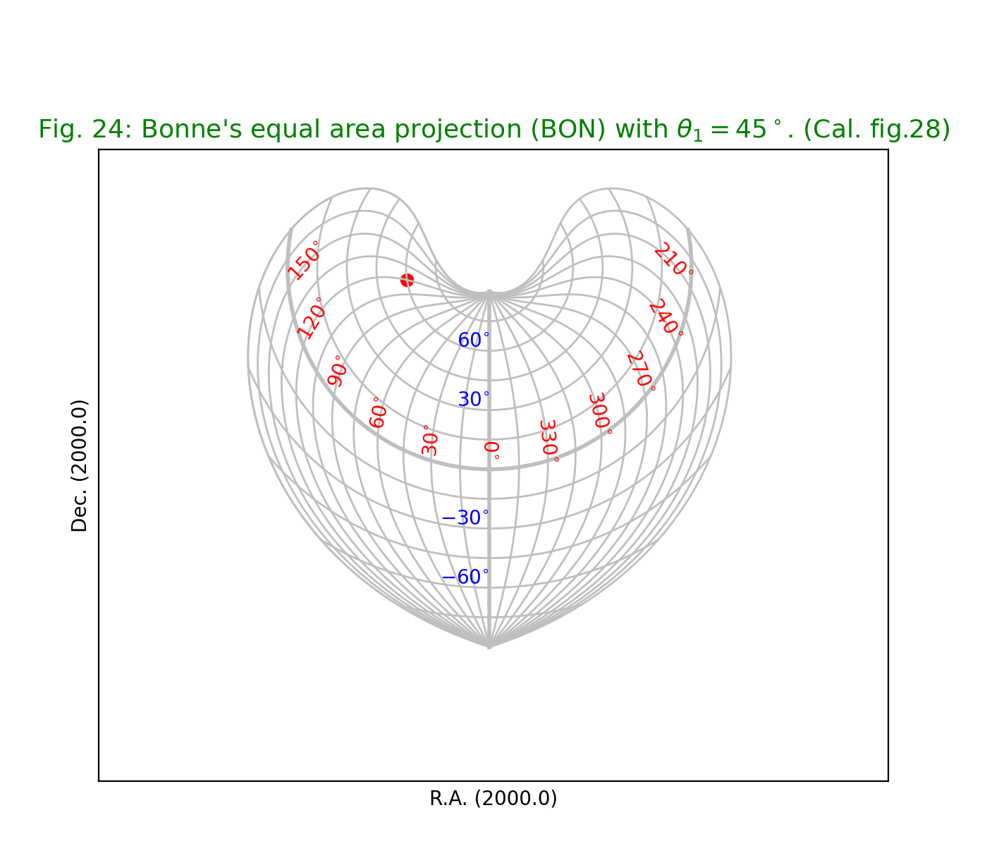
Fig.24: Bonne’s equal area projection (BON)
from kapteyn import maputils
import numpy
from service import *

fignum = 24
fig = plt.figure(figsize=figsize)
frame = fig.add_axes(plotbox)
theta1 = 45
title = r"Bonne's equal area projection (BON) with $\theta_1=45^\circ$. (Cal. fig.28)"
header = {'NAXIS'  : 2, 'NAXIS1': 100, 'NAXIS2': 80,
          'CTYPE1' : 'RA---BON',
          'CRVAL1' : 0.0, 'CRPIX1' : 50, 'CUNIT1' : 'deg', 'CDELT1' : -4.0,
          'CTYPE2' : 'DEC--BON',
          'CRVAL2' : 0.0, 'CRPIX2' : 40, 'CUNIT2' : 'deg', 'CDELT2' : 4.0,
          'PV2_1'  : theta1
         }
X = polrange()
Y = numpy.arange(-75,90,15.0)
f = maputils.FITSimage(externalheader=header)
annim = f.Annotatedimage(frame)
grat = annim.Graticule(axnum= (1,2), wylim=(-90,90.0), wxlim=(0,360),
                       startx=X, starty=Y)
grat.setp_lineswcs0(0, lw=2)
grat.setp_lineswcs1(0, lw=2)
w1 = numpy.arange(0,151,30.0)
w2 = numpy.arange(210,360,30.0)
lon_world = numpy.concatenate((w1, w2))
lat_world = [-60, -30, 30, 60]
lat_constval = 10
labkwargs0 = {'color':'r', 'va':'center', 'ha':'center'}
labkwargs1 = {'color':'b', 'va':'bottom', 'ha':'right'}
doplot(frame, fignum, annim, grat, title,
       lon_world=lon_world, lat_world=lat_world,
       labkwargs0=labkwargs0, labkwargs1=labkwargs1,
       lat_constval=lat_constval, markerpos=markerpos)
(Source code, png, hires.png, pdf)
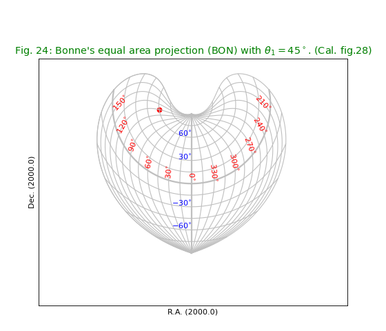
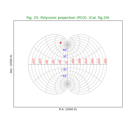
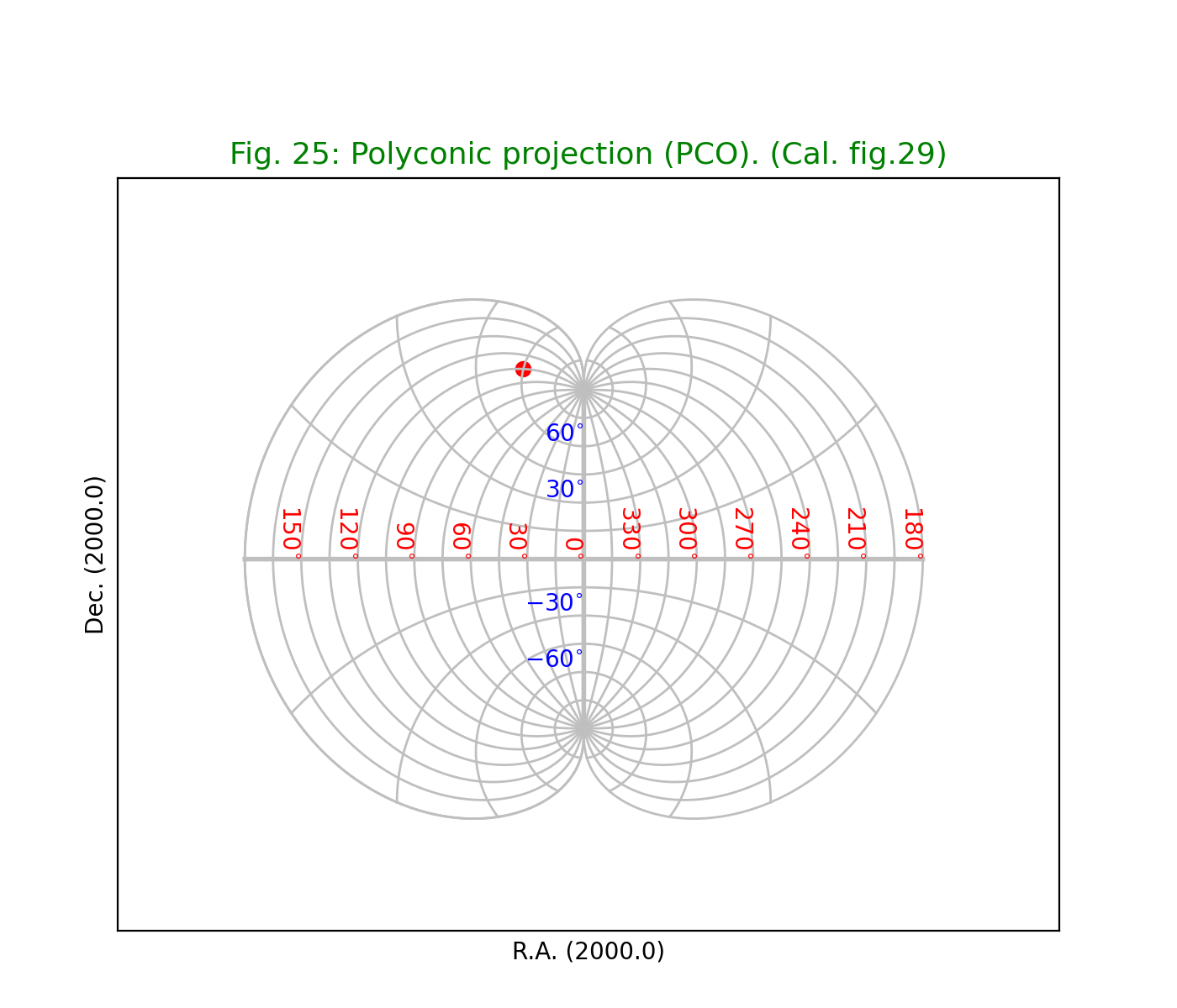
Fig.25: Polyconic projection (PCO)
Near the poles we have a problem to draw graticule lines at constant latitude. With the defaults for the Graticule constructor we would observe a horizontal line that connects longitudes -180 and 180 deg. near the poles. From a plotting point of view the range -180 to 180 deg. means a closed shape (e.g. a circle near a pole). To prevent horizontal jumps in such plots we defined a jump in terms of pixels. If the distance between two points is much bigger than the pixel sampling then it must be a jump. However, in some projections (like this one), the jump near the pole becomes so small that we cannot avoid a horizontal connection. By increasing the number of samples in parameter gridsamples we force the size of a jump relatively to be bigger. With a value gridsamples=2000 we avoid the unwanted connections.
The reason that sometimes line sections are connected which
are not supposed to be connected has to
do with the fact that in wcsgrat the range in world coordinates is increased a little
bit to be sure we cross borders so that we are able to plot
ticks. But in the gaps (see the plot below) this can result in the fact that we start
to sample on the wrong side of the gap. Then there is a gap
and the sampling continues on the other side of the gap. The algorithm
thinks these points should be connected because the gap is too small
to be detected as a jump.
Note that we could also have decreased the size of the range
in world coordinates in longitude (e.g. wxlim=(-179.9, 179.9)) but this
results in small gaps near all borders.
from kapteyn import maputils
import numpy
from service import *

fignum = 25
fig = plt.figure(figsize=figsize)
frame = fig.add_axes(plotbox)
title = r"Polyconic projection (PCO). (Cal. fig.29)"
header = {'NAXIS'  : 2, 'NAXIS1': 100, 'NAXIS2': 80,
          'CTYPE1' : 'RA---PCO',
          'CRVAL1' : 0.0, 'CRPIX1' : 50, 'CUNIT1' : 'deg', 'CDELT1' : -5.0,
          'CTYPE2' : 'DEC--PCO',
          'CRVAL2' : 0.0, 'CRPIX2' : 40, 'CUNIT2' : 'deg', 'CDELT2' : 5.0
         }
X = polrange()
Y = numpy.arange(-75,90,15.0)
# !!!!!! Let the world coordinates for constant latitude run from 180,180
# instead of 0,360. Then one prevents the connection between the two points
# 179.9999 and 180.0001 which is a jump, but smaller than the definition of
# a rejected jump in the wcsgrat module.
# Also we need to increase the value of 'gridsamples' to
# increase the relative size of a jump.
f = maputils.FITSimage(externalheader=header)
annim = f.Annotatedimage(frame)
grat = annim.Graticule(axnum= (1,2),
                       wylim=(-90,90.0), wxlim=(-180,180),
                       startx=X, starty=Y, gridsamples=2000)
grat.setp_lineswcs0(0, lw=2)
grat.setp_lineswcs1(0, lw=2)
# Remove the left 180 deg and print the right 180 deg instead
w1 = numpy.arange(0,151,30.0)
w2 = numpy.arange(180,360,30.0)
w2[0] = 180 + epsilon
lon_world = numpy.concatenate((w1, w2))
lat_world = [-60, -30, 30, 60]
labkwargs0 = {'color':'r', 'va':'bottom', 'ha':'right'}
labkwargs1 = {'color':'b', 'va':'bottom', 'ha':'right'}
doplot(frame, fignum, annim, grat, title,
       lon_world=lon_world, lat_world=lat_world,
       labkwargs0=labkwargs0, labkwargs1=labkwargs1,
       markerpos=markerpos)
(Source code, png, hires.png, pdf)

Quad cube projections projections
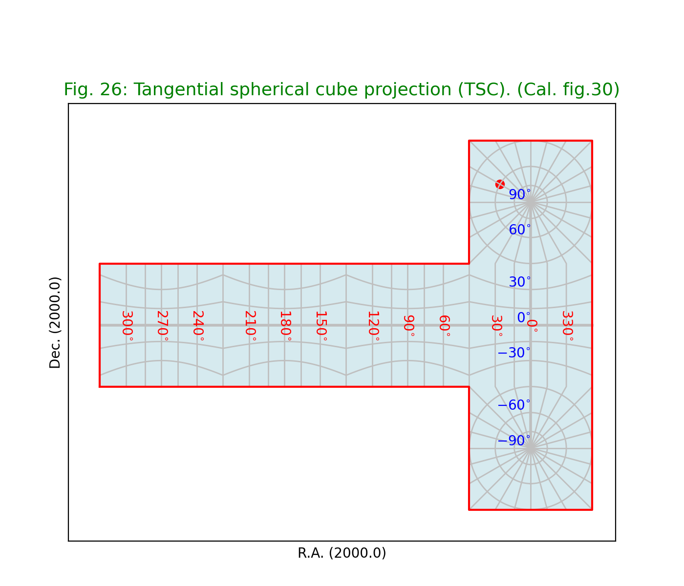
Fig.26: Tangential spherical cube projection (TSC)
For all the quad cube projections we plotted a border by converting edges in world coordinates into pixel coordinates and connected them in the right order.
from kapteyn import maputils
import numpy
from service import *

fignum = 26
fig = plt.figure(figsize=figsize)
frame = fig.add_axes(plotbox)
title = r"Tangential spherical cube projection (TSC). (Cal. fig.30)"
header = {'NAXIS'  : 2, 'NAXIS1': 100, 'NAXIS2': 80,
          'CTYPE1' : 'RA---TSC',
          'CRVAL1' : 0.0, 'CRPIX1' : 85, 'CUNIT1' : 'deg', 'CDELT1' : -4.0,
          'CTYPE2' : 'DEC--TSC',
          'CRVAL2' : 0.0, 'CRPIX2' : 40, 'CUNIT2' : 'deg', 'CDELT2' : 4.0
         }
X = numpy.arange(0,370.0,15.0)
Y = numpy.arange(-75,90,15.0)
f = maputils.FITSimage(externalheader=header)
annim = f.Annotatedimage(frame)
grat = annim.Graticule(axnum= (1,2), wylim=(-90,90.0), wxlim=(-180,180),
                       startx=X, starty=Y)
grat.setp_lineswcs0(0, lw=2)
grat.setp_lineswcs1(0, lw=2)
# Make a polygon for the border
perimeter = getperimeter(grat)
lon_world = list(range(0,360,30))
lat_world = [-dec0, -60, -30, 0, 30, 60, dec0]
labkwargs0 = {'color':'r', 'va':'center', 'ha':'center'}
labkwargs1 = {'color':'b', 'va':'bottom', 'ha':'right'}
doplot(frame, fignum, annim, grat, title,
       lon_world=lon_world, lat_world=lat_world,
       labkwargs0=labkwargs0, labkwargs1=labkwargs1,
       perimeter=perimeter, markerpos=markerpos)
(Source code, png, hires.png, pdf)

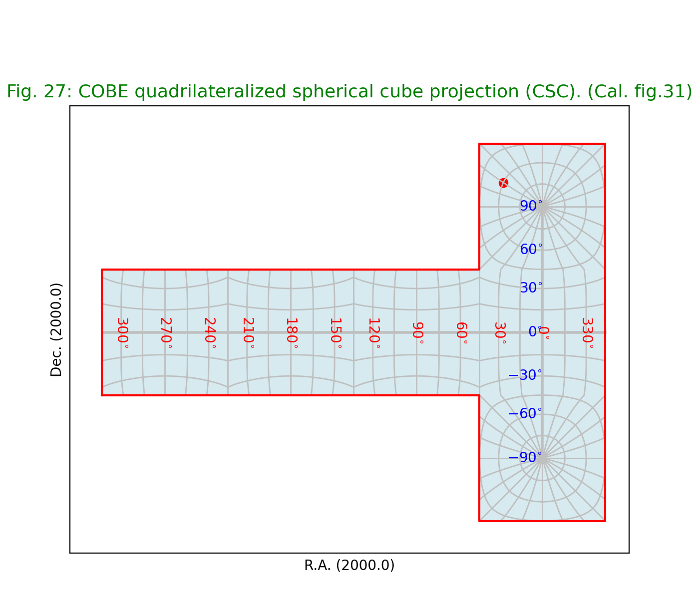
Fig.27: COBE quadrilateralized spherical cube projection (CSC)
from kapteyn import maputils
import numpy
from service import *

fignum = 27
fig = plt.figure(figsize=figsize)
frame = fig.add_axes(plotbox)
title = r"COBE quadrilateralized spherical cube projection (CSC). (Cal. fig.31)"
header = {'NAXIS'  : 2, 'NAXIS1': 100, 'NAXIS2': 80,
          'CTYPE1' : 'RA---CSC',
          'CRVAL1' : 0.0, 'CRPIX1' : 85, 'CUNIT1' : 'deg', 'CDELT1' : -4.0,
          'CTYPE2' : 'DEC--CSC',
          'CRVAL2' : 0.0, 'CRPIX2' : 40, 'CUNIT2' : 'deg', 'CDELT2' : 4.0
         }
X = numpy.arange(0,370.0,15.0)
Y = numpy.arange(-75,90,15.0)
f = maputils.FITSimage(externalheader=header)
annim = f.Annotatedimage(frame)
grat = annim.Graticule(axnum= (1,2), wylim=(-90,90.0), wxlim=(-180,180),
                       startx=X, starty=Y)
grat.setp_lineswcs0(0, lw=2)
grat.setp_lineswcs1(0, lw=2)
# Make a polygon for the border
perimeter = getperimeter(grat)
lon_world = list(range(0,360,30))
lat_world = [-dec0, -60, -30, 0, 30, 60, dec0]
labkwargs0 = {'color':'r', 'va':'center', 'ha':'center'}
labkwargs1 = {'color':'b', 'va':'center', 'ha':'right'}
doplot(frame, fignum, annim, grat, title,
       lon_world=lon_world, lat_world=lat_world,
       labkwargs0=labkwargs0, labkwargs1=labkwargs1,
       perimeter=perimeter, markerpos=markerpos)
(Source code, png, hires.png, pdf)
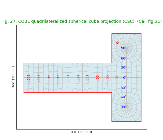
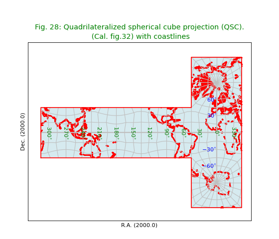
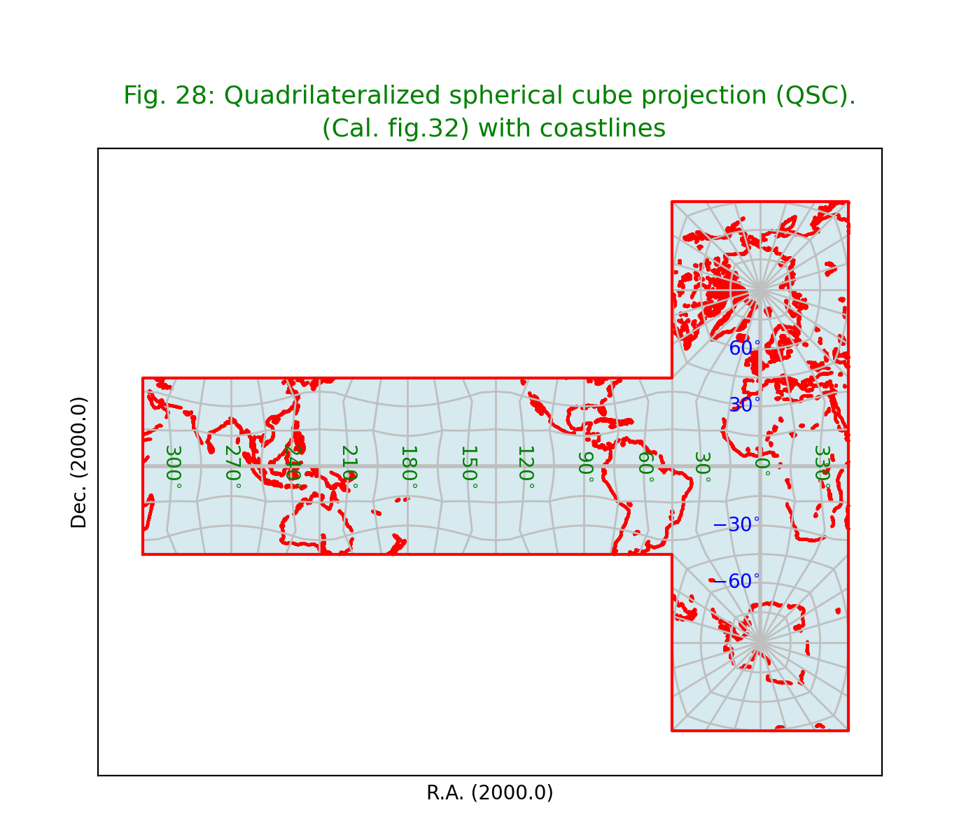
Fig.28: Quadrilateralized spherical cube projection (QSC)
from kapteyn import maputils
import numpy
from service import *

fignum = 28
fig = plt.figure(figsize=figsize)
frame = fig.add_axes(plotbox)
title = r"""Quadrilateralized spherical cube projection (QSC).
 (Cal. fig.32) with coastlines"""
header = {'NAXIS'  : 2, 'NAXIS1': 100, 'NAXIS2': 80,
          'CTYPE1' : 'RA---QSC',
          'CRVAL1' : 0.0, 'CRPIX1' : 85, 'CUNIT1' : 'deg', 'CDELT1' : -4.0,
          'CTYPE2' : 'DEC--QSC',
          'CRVAL2' : 0.0, 'CRPIX2' : 40, 'CUNIT2' : 'deg', 'CDELT2' : 4.0,
         }
X = numpy.arange(-180,180,15)
Y = numpy.arange(-75,90,15.0)
f = maputils.FITSimage(externalheader=header)
annim = f.Annotatedimage(frame)
grat = annim.Graticule(axnum= (1,2), wylim=(-90,90.0), wxlim=(0,360),
                       startx=X, starty=Y)
grat.setp_lineswcs0(0, lw=2)
grat.setp_lineswcs1(0, lw=2)
lon_world = list(range(0,360,30))
lat_world = [-60, -30, 30, 60]
perimeter = getperimeter(grat)
labkwargs0 = {'color':'g', 'va':'center', 'ha':'center'}
labkwargs1 = {'color':'b', 'va':'center', 'ha':'right'}
doplot(frame, fignum, annim, grat, title,
       lon_world=lon_world, lat_world=lat_world,
       labkwargs0=labkwargs0, labkwargs1=labkwargs1,
       perimeter=perimeter, plotdata=True)
(Source code, png, hires.png, pdf)

Oblique projections
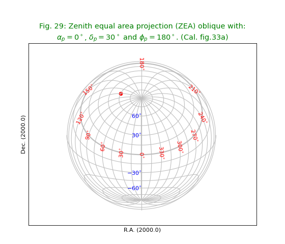
Fig.29: Zenith equal area projection (ZEA) oblique
from kapteyn import maputils
import numpy
from service import *

fignum = 29
fig = plt.figure(figsize=figsize)
frame = fig.add_axes(plotbox)
title = r"""Zenith equal area projection (ZEA) oblique with:
$\alpha_p=0^\circ$, $\delta_p=30^\circ$ and $\phi_p=180^\circ$. (Cal. fig.33a)"""
header = {'NAXIS' : 2, 'NAXIS1': 100, 'NAXIS2': 80,
          'CTYPE1' : 'RA---ZEA',
          'CRVAL1' : 0.0, 'CRPIX1' : 50, 'CUNIT1' : 'deg', 'CDELT1' : -3.5,
          'CTYPE2' : 'DEC--ZEA',
          'CRVAL2' : 30.0, 'CRPIX2' : 40, 'CUNIT2' : 'deg', 'CDELT2' : 3.5,
         }
X = numpy.arange(0,360,15.0)
Y = numpy.arange(-75,90,15.0)
f = maputils.FITSimage(externalheader=header)
annim = f.Annotatedimage(frame)
grat = annim.Graticule(axnum= (1,2), wylim=(-90,90.0), wxlim=(0,360),
                       startx=X, starty=Y)
grat.setp_lineswcs0(0, lw=2)
grat.setp_lineswcs1(0, lw=2)
lon_world = list(range(0,360,30))
lat_world = [-60, -30, 30, 60]
labkwargs0 = {'color':'r', 'va':'center', 'ha':'center'}
labkwargs1 = {'color':'b', 'va':'center', 'ha':'right'}
doplot(frame, fignum, annim, grat, title,
       lon_world=lon_world, lat_world=lat_world,
       labkwargs0=labkwargs0, labkwargs1=labkwargs1,
       markerpos=markerpos)
(Source code, png, hires.png, pdf)

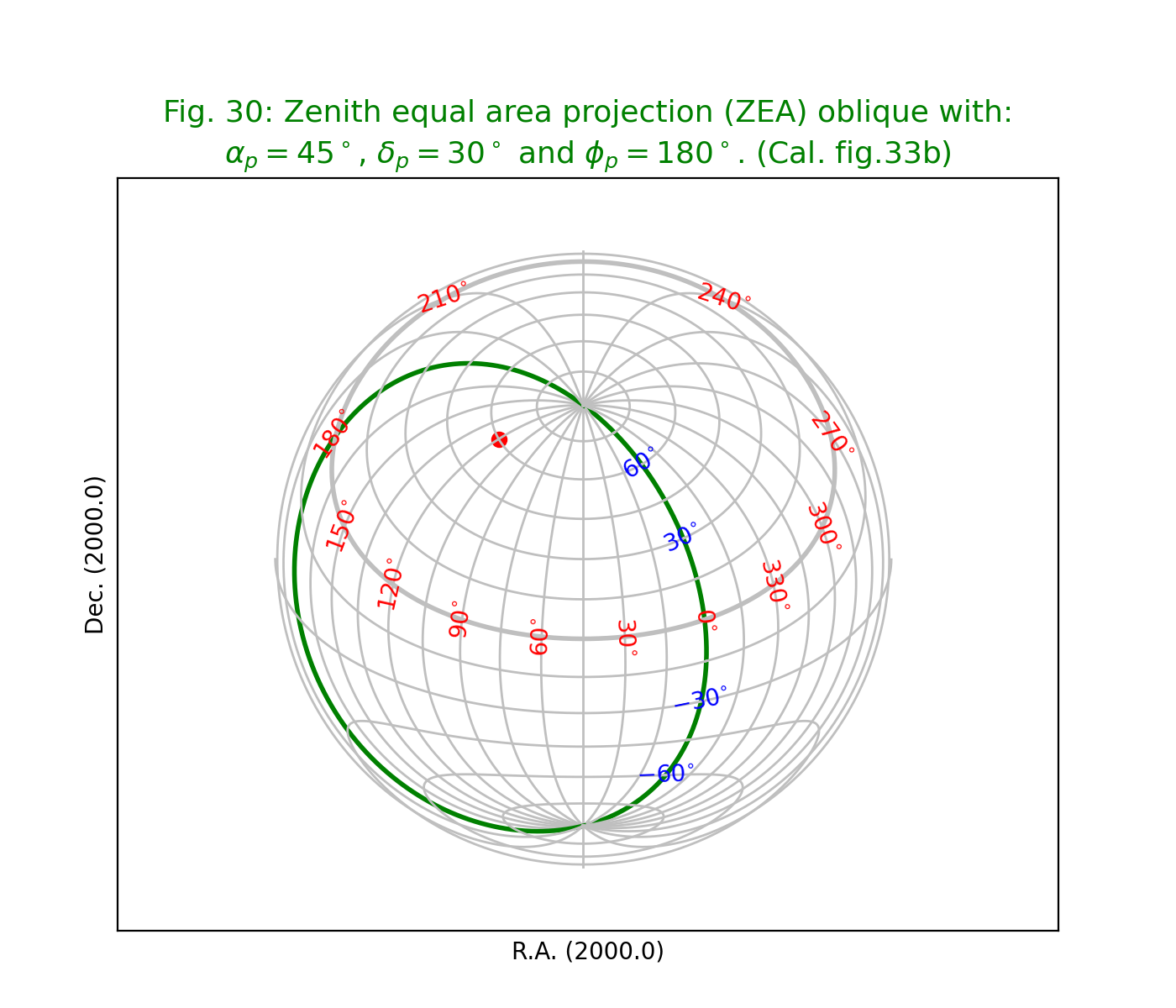
Fig.30: Zenith equal area projection (ZEA) oblique
from kapteyn import maputils
import numpy
from service import *

fignum = 30
fig = plt.figure(figsize=figsize)
frame = fig.add_axes(plotbox)
title = r"""Zenith equal area projection (ZEA) oblique with:
$\alpha_p=45^\circ$, $\delta_p=30^\circ$ and $\phi_p=180^\circ$. (Cal. fig.33b)"""
header = {'NAXIS' : 2, 'NAXIS1': 100, 'NAXIS2': 80,
          'CTYPE1' : 'RA---ZEA',
          'CRVAL1' :45.0, 'CRPIX1' : 50, 'CUNIT1' : 'deg', 'CDELT1' : -3.5,
          'CTYPE2' : 'DEC--ZEA',
          'CRVAL2' : 30.0, 'CRPIX2' : 40, 'CUNIT2' : 'deg', 'CDELT2' : 3.5
         }
X = numpy.arange(0,360.0,15.0)
Y = numpy.arange(-75,90,15.0)
f = maputils.FITSimage(externalheader=header)
annim = f.Annotatedimage(frame)
grat = annim.Graticule(axnum= (1,2), wylim=(-90,90.0), wxlim=(0,360),
                       startx=X, starty=Y)
grat.setp_lineswcs0((0,180), color='g', lw=2)
grat.setp_lineswcs1(0, lw=2)
lon_world = list(range(0,360,30))
lat_world = [-60, -30, 30, 60]
labkwargs0 = {'color':'r', 'va':'center', 'ha':'center'}
labkwargs1 = {'color':'b', 'va':'center', 'ha':'center'}
deltapy0 = 0 #2
doplot(frame, fignum, annim, grat, title,
       lon_world=lon_world, lat_world=lat_world,
       labkwargs0=labkwargs0, labkwargs1=labkwargs1,
       deltapy0=deltapy0, markerpos=markerpos)
(Source code, png, hires.png, pdf)

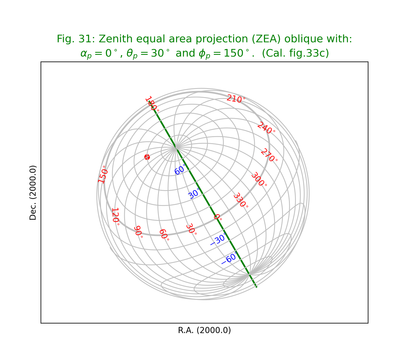
Fig.31: Zenith equal area projection (ZEA) oblique with PV1_3 element
from kapteyn import maputils
import numpy
from service import *

fignum = 31
fig = plt.figure(figsize=figsize)
frame = fig.add_axes(plotbox)
title = r"""Zenith equal area projection (ZEA) oblique with:
$\alpha_p=0^\circ$, $\theta_p=30^\circ$ and $\phi_p = 150^\circ$.  (Cal. fig.33c)"""
header = {'NAXIS' : 2, 'NAXIS1': 100, 'NAXIS2': 80,
          'CTYPE1' : 'RA---ZEA',
          'CRVAL1' : 0.0, 'CRPIX1' : 50, 'CUNIT1' : 'deg', 'CDELT1' : -3.5,
          'CTYPE2' : 'DEC--ZEA',
          'CRVAL2' : 30.0, 'CRPIX2' : 40, 'CUNIT2' : 'deg', 'CDELT2' : 3.5,
          'PV1_3' : 150.0    # Works only with patched WCSLIB 4.3
         }
X = numpy.arange(0,360.0,15.0)
Y = numpy.arange(-75,90,15.0)
f = maputils.FITSimage(externalheader=header)
annim = f.Annotatedimage(frame)
grat = annim.Graticule(axnum= (1,2), wylim=(-90,90.0), wxlim=(0,360),
                       startx=X, starty=Y)
grat.setp_lineswcs0((0,180), color='g', lw=2)
grat.setp_lineswcs1(0, lw=2)
lon_world = list(range(0,360,30))
lat_world = [-60, -30, 30, 60]
labkwargs0 = {'color':'r', 'va':'center', 'ha':'center'}
labkwargs1 = {'color':'b', 'va':'center', 'ha':'right'}
doplot(frame, fignum, annim, grat, title,
       lon_world=lon_world, lat_world=lat_world,
       labkwargs0=labkwargs0, labkwargs1=labkwargs1,
       markerpos=markerpos)
(Source code, png, hires.png, pdf)
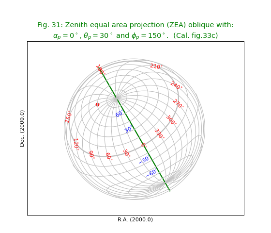
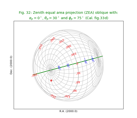
Fig.32: Zenith equal area projection (ZEA) oblique with PV1_3 element II
from kapteyn import maputils
import numpy
from service import *

fignum = 32
fig = plt.figure(figsize=figsize)
frame = fig.add_axes(plotbox)
title = r"""Zenith equal area projection (ZEA) oblique with:
$\alpha_p=0^\circ$, $\theta_p=30^\circ$ and $\phi_p = 75^\circ$ (Cal. fig.33d)"""
header = {'NAXIS' : 2, 'NAXIS1': 100, 'NAXIS2': 80,
          'CTYPE1' : 'RA---ZEA',
          'CRVAL1' : 0.0, 'CRPIX1' : 50, 'CUNIT1' : 'deg', 'CDELT1' : -3.5,
          'CTYPE2' : 'DEC--ZEA',
          'CRVAL2' : 30.0, 'CRPIX2' : 40, 'CUNIT2' : 'deg', 'CDELT2' : 3.5,
          'PV1_3' : 75.0
         }
X = numpy.arange(0,360.0,15.0)
Y = numpy.arange(-75,90,15.0)
f = maputils.FITSimage(externalheader=header)
annim = f.Annotatedimage(frame)
grat = annim.Graticule(axnum= (1,2), wylim=(-90,90.0), wxlim=(0,360),
                       startx=X, starty=Y)
grat.setp_lineswcs0((0,180), color='g', lw=2)
grat.setp_lineswcs1(0, lw=2)
lon_world = list(range(0,360,30))
lat_world = [-60, -30, 30, 60]
addangle0 = 180
labkwargs0 = {'color':'r', 'va':'center', 'ha':'center'}
labkwargs1 = {'color':'b', 'va':'center', 'ha':'center'}
doplot(frame, fignum, annim, grat, title,
       lon_world=lon_world, lat_world=lat_world,
       labkwargs0=labkwargs0, labkwargs1=labkwargs1,
       addangle0=addangle0, markerpos=markerpos)
(Source code, png, hires.png, pdf)

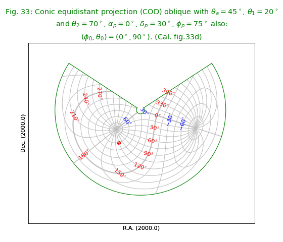
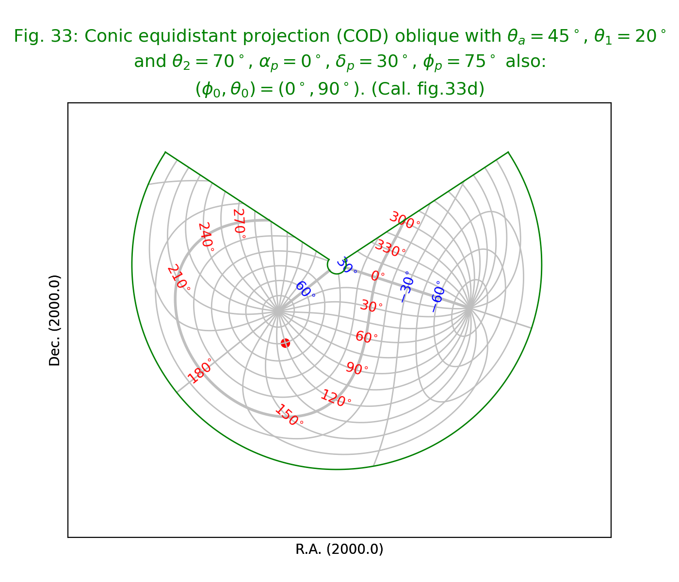
Fig.33: Conic equidistant projection (COD) oblique
from kapteyn import maputils
import numpy
from service import *

fignum = 33
fig = plt.figure(figsize=figsize)
frame = fig.add_axes(plotbox)
theta_a = 45.0
t1 = 20.0; t2 = 70.0
eta = abs(t1-t2)/2.0
title = r"""Conic equidistant projection (COD) oblique with $\theta_a=45^\circ$, $\theta_1=20^\circ$
and $\theta_2=70^\circ$, $\alpha_p = 0^\circ$, $\delta_p = 30^\circ$, $\phi_p = 75^\circ$ also:
$(\phi_0,\theta_0) = (0^\circ,90^\circ)$. (Cal. fig.33d)"""
header = {'NAXIS'  : 2, 'NAXIS1': 100, 'NAXIS2': 80,
          'CTYPE1' : 'RA---COD',
          'CRVAL1' : 0, 'CRPIX1' : 50, 'CUNIT1' : 'deg', 'CDELT1' : -5.0,
          'CTYPE2' : 'DEC--COD',
          'CRVAL2' : 30, 'CRPIX2' : 40, 'CUNIT2' : 'deg', 'CDELT2' : 5.0,
          'PV2_1'  : theta_a,
          'PV2_2' :  eta,
          'PV1_1'  : 0.0, 'PV1_2' : 90.0,  # IMPORTANT. This is a setting from section 7.1, p 1103
          'LONPOLE' :75.0
         }
X = numpy.arange(0,370.0,15.0);  X[-1] = 180.000001
Y = numpy.arange(-75,90,15.0)
f = maputils.FITSimage(externalheader=header)
annim = f.Annotatedimage(frame)
grat = annim.Graticule(axnum= (1,2), wylim=(-90,90.0), wxlim=(0,360),
                       startx=X, starty=Y)
grat.setp_lineswcs0(0, lw=2)
grat.setp_lineswcs1(0, lw=2)
# Draw border with standard graticule
header['CRVAL1'] = 0.0
header['CRVAL2'] = theta_a
header['LONPOLE'] = 0.0
del header['PV1_1']
del header['PV1_2']
# Non oblique version as border
border = annim.Graticule(header, axnum= (1,2), wylim=(-90,90.0), wxlim=(-180,180),
                         startx=(180-epsilon, -180+epsilon), starty=(-90,90))
border.setp_lineswcs0(color='g')   # Show borders in different color
border.setp_lineswcs1(color='g')
lon_world = list(range(0,360,30))
lat_world = [-60, -30, 30, 60]
labkwargs0 = {'color':'r', 'va':'center', 'ha':'center'}
labkwargs1 = {'color':'b', 'va':'center', 'ha':'center'}
doplot(frame, fignum, annim, grat, title,
       lon_world=lon_world, lat_world=lat_world,
       labkwargs0=labkwargs0, labkwargs1=labkwargs1,
       markerpos=markerpos)
(Source code, png, hires.png, pdf)

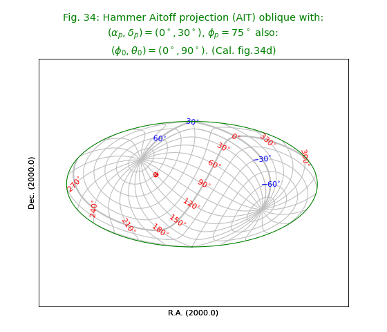
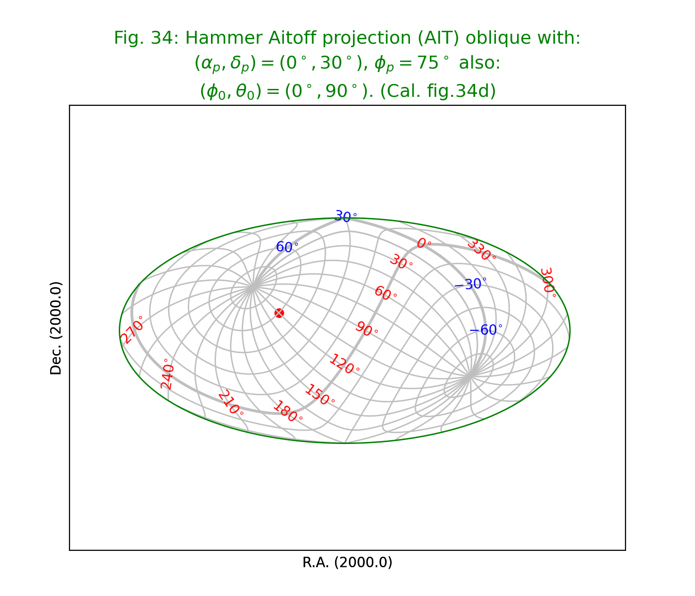
Fig.34: Hammer Aitoff projection (AIT) oblique
from kapteyn import maputils
import numpy
from service import *

fignum = 34
fig = plt.figure(figsize=figsize)
frame = fig.add_axes(plotbox)
title = r"""Hammer Aitoff projection (AIT) oblique with:
$(\alpha_p,\delta_p) = (0^\circ,30^\circ)$, $\phi_p = 75^\circ$ also:
$(\phi_0,\theta_0) = (0^\circ,90^\circ)$. (Cal. fig.34d)"""
# Header works only with a patched wcslib 4.3
header = {'NAXIS'  : 2, 'NAXIS1': 100, 'NAXIS2': 80,
          'CTYPE1' : 'RA---AIT',
          'CRVAL1' : 0.0, 'CRPIX1' : 50, 'CUNIT1' : 'deg', 'CDELT1' : -4.0,
          'CTYPE2' : 'DEC--AIT',
          'CRVAL2' : 30.0, 'CRPIX2' : 40, 'CUNIT2' : 'deg', 'CDELT2' : 4.0,
          'LONPOLE' :75.0,
          'PV1_1'  : 0.0, 'PV1_2' : 90.0,  # IMPORTANT. This is a setting from Cal.section 7.1, p 1103
         }
X = numpy.arange(0,390.0,15.0);
Y = numpy.arange(-75,90,15.0)
f = maputils.FITSimage(externalheader=header)
annim = f.Annotatedimage(frame)
grat = annim.Graticule(axnum= (1,2), wylim=(-90,90.0), wxlim=(0,360),
                       startx=X, starty=Y)
grat.setp_lineswcs0(0, lw=2)
grat.setp_lineswcs1(0, lw=2)
# Draw border with standard graticule
header['CRVAL1'] = 0.0
header['CRVAL2'] = 0.0
del header['PV1_1']
del header['PV1_2']
header['LONPOLE'] = 0.0
header['LATPOLE'] = 0.0
border = annim.Graticule(header, axnum= (1,2), wylim=(-90,90.0), wxlim=(-180,180),
                         startx=(180-epsilon, -180+epsilon), skipy=True)
border.setp_lineswcs0(color='g')   # Show borders in different color
border.setp_lineswcs1(color='g')
lon_world = list(range(0,360,30))
lat_world = [-60, -30, 30, 60]
labkwargs0 = {'color':'r', 'va':'center', 'ha':'center'}
labkwargs1 = {'color':'b', 'va':'center', 'ha':'center'}
doplot(frame, fignum, annim, grat, title,
       lon_world=lon_world, lat_world=lat_world,
       labkwargs0=labkwargs0, labkwargs1=labkwargs1,
       markerpos=markerpos)
(Source code, png, hires.png, pdf)

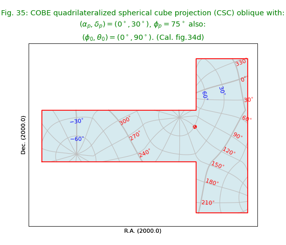
Fig.35: COBE quadrilateralized spherical cube projection (CSC) oblique
from kapteyn import maputils
import numpy
from service import *

fignum = 35
fig = plt.figure(figsize=figsize)
frame = fig.add_axes(plotbox)
title = r"""COBE quadrilateralized spherical cube projection (CSC) oblique with:
$(\alpha_p,\delta_p) = (0^\circ,30^\circ)$, $\phi_p = 75^\circ$ also:
$(\phi_0,\theta_0) = (0^\circ,90^\circ)$. (Cal. fig.34d)"""
header = {'NAXIS'  : 2, 'NAXIS1': 100, 'NAXIS2': 80,
          'CTYPE1' : 'RA---CSC',
          'CRVAL1' : 0.0, 'CRPIX1' : 85, 'CUNIT1' : 'deg', 'CDELT1' : -4.0,
          'CTYPE2' : 'DEC--CSC',
          'CRVAL2' : 30.0, 'CRPIX2' : 40, 'CUNIT2' : 'deg', 'CDELT2' : 4.0,
          'LONPOLE': 75.0,
          'PV1_1'  : 0.0, 'PV1_2' : 90.0,
         }
X = numpy.arange(0,370.0,30.0)
Y = numpy.arange(-60,90,30.0)
f = maputils.FITSimage(externalheader=header)
annim = f.Annotatedimage(frame)
grat = annim.Graticule(axnum= (1,2), wylim=(-90,90.0), wxlim=(-180,180),
                       startx=X, starty=Y)
grat.setp_lineswcs0(0, lw=2)
grat.setp_lineswcs1(0, lw=2)
# Take border from non-oblique version
header['CRVAL2'] = 0.0
del header['PV1_1']
del header['PV1_2']
del header['LONPOLE']
border = annim.Graticule(header, axnum= (1,2), wylim=(-90,90.0), wxlim=(-180,180),
                         skipx=True, skipy=True)
perimeter = getperimeter(border)
lon_world = list(range(0,360,30))
lat_world = [-60, -30, 30, 60]
labkwargs0 = {'color':'r', 'va':'center', 'ha':'left'}
labkwargs1 = {'color':'b', 'va':'top', 'ha':'center'}
doplot(frame, fignum, annim, grat, title,
       lon_world=lon_world, lat_world=lat_world,
       labkwargs0=labkwargs0, labkwargs1=labkwargs1,
       perimeter=perimeter, markerpos=markerpos)
(Source code, png, hires.png, pdf)

Miscellaneous
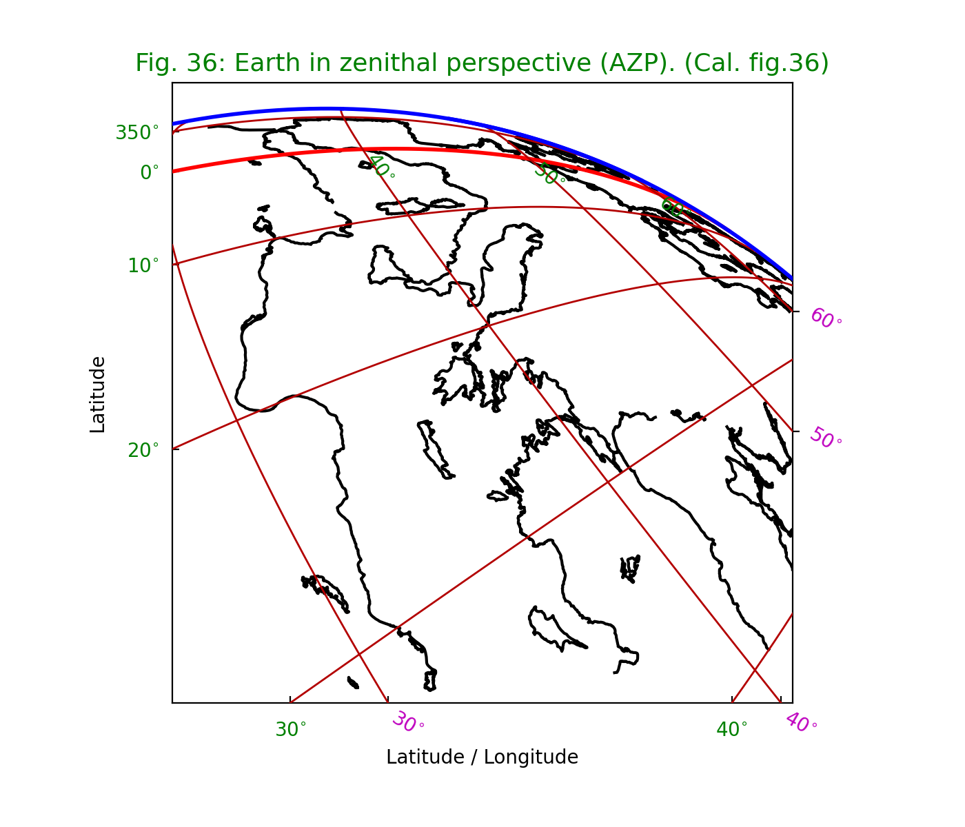
Fig.36: Earth in zenithal perspective (AZP)
The coastline used in this example is read from file
world.txt which is composed
from a plain text version of the CIA World DataBank II map database
made by Dave Pape (http://www.evl.uic.edu/pape/data/WDB/).
We used values ‘TLON’, ‘TLAT’ for the CTYPE’s.
These are recognized by WCSLIB as longitude and latitude.
Any other prefix is also valid.
Note the intensive use of methods to set label/tick- and plot properties.
wcsgrat.Graticule.setp_lineswcs0(),
wcsgrat.Graticule.setp_lineswcs1(),
wcsgrat.Graticule.setp_tick()and
wcsgrat.Graticule.setp_linespecial()
from kapteyn import maputils
import numpy
from service import *

fignum = 36
fig = plt.figure(figsize=figsize)
frame = fig.add_axes((0.1,0.15,0.8,0.75))
title = 'Earth in zenithal perspective (AZP). (Cal. fig.36)'
# The ctype's are TLON, TLAT. These are recognized by WCSlib as longitude and latitude.
# Any other prefix is also valid.
header = {'NAXIS'  : 2, 'NAXIS1': 2048, 'NAXIS2': 2048,
          'PC1_1' : 0.9422, 'PC1_2' : -0.3350,
          'PC2_1' : 0.3350, 'PC2_2' : 0.9422,
          'CTYPE1' : 'TLON-AZP',
          'CRVAL1' : 31.15, 'CRPIX1' : 681.67, 'CUNIT1' : 'deg', 'CDELT1' : 0.008542,
          'CTYPE2' : 'TLAT-AZP',
          'CRVAL2' : 30.03, 'CRPIX2' : 60.12, 'CUNIT2' : 'deg', 'CDELT2' : 0.008542,
          'PV2_1' : -1.350, 'PV2_2' : 25.8458,
          'LONPOLE' : 143.3748,
         }
X = numpy.arange(-30,60.0,10.0)
Y = numpy.arange(-40,65,10.0)
f = maputils.FITSimage(externalheader=header)
annim = f.Annotatedimage(frame)
grat = annim.Graticule(axnum= (1,2), wylim=(-30,90.0), wxlim=(-20,60),
                       startx=X, starty=Y, gridsamples=4000)
grat.setp_lineswcs1(color='#B30000')
grat.setp_lineswcs0(color='#B30000')
grat.setp_lineswcs0(0, color='r', lw=2)
grat.setp_plotaxis('bottom', mode='all_ticks', label='Latitude / Longitude')
grat.setp_plotaxis('left', mode='switched_ticks', label='Latitude')
grat.setp_plotaxis('right', mode='native_ticks')
grat.setp_tick(wcsaxis=0, color='g', fmt="Dms")
grat.setp_tick(wcsaxis=1, color='m', fmt="Dms")
grat.setp_tick(wcsaxis=1, plotaxis=('bottom','right'), color='m', rotation=-30, ha='left')
grat.setp_tick(plotaxis='left', position=-10, visible=False)
g = grat.scanborder(560, 1962, 2)
grat.setp_linespecial(g, color='b', lw=2)
lat_world = lon_world = []
drawgrid = True
markerpos = None
# Proof that WCSlib thinks TLON, TLAT are valid longitudes & latitudes
print("TLON and TLAT are recognized as:", grat.gmap.types)
labkwargs0 = {'color':'r', 'va':'center', 'ha':'center'}
labkwargs1 = {'color':'g', 'va':'top', 'ha':'left'}
doplot(frame, fignum, annim, grat, title,
       lon_fmt="Dms", lat_fmt="Dms",
       labkwargs0=labkwargs0, labkwargs1=labkwargs1,
       plotdata=True, markerpos=markerpos)
(Source code, png, hires.png, pdf)
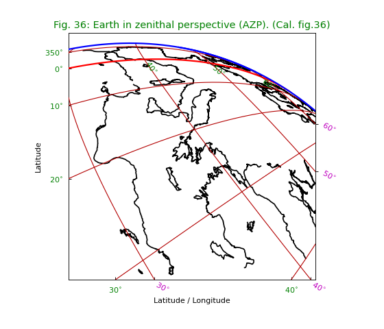
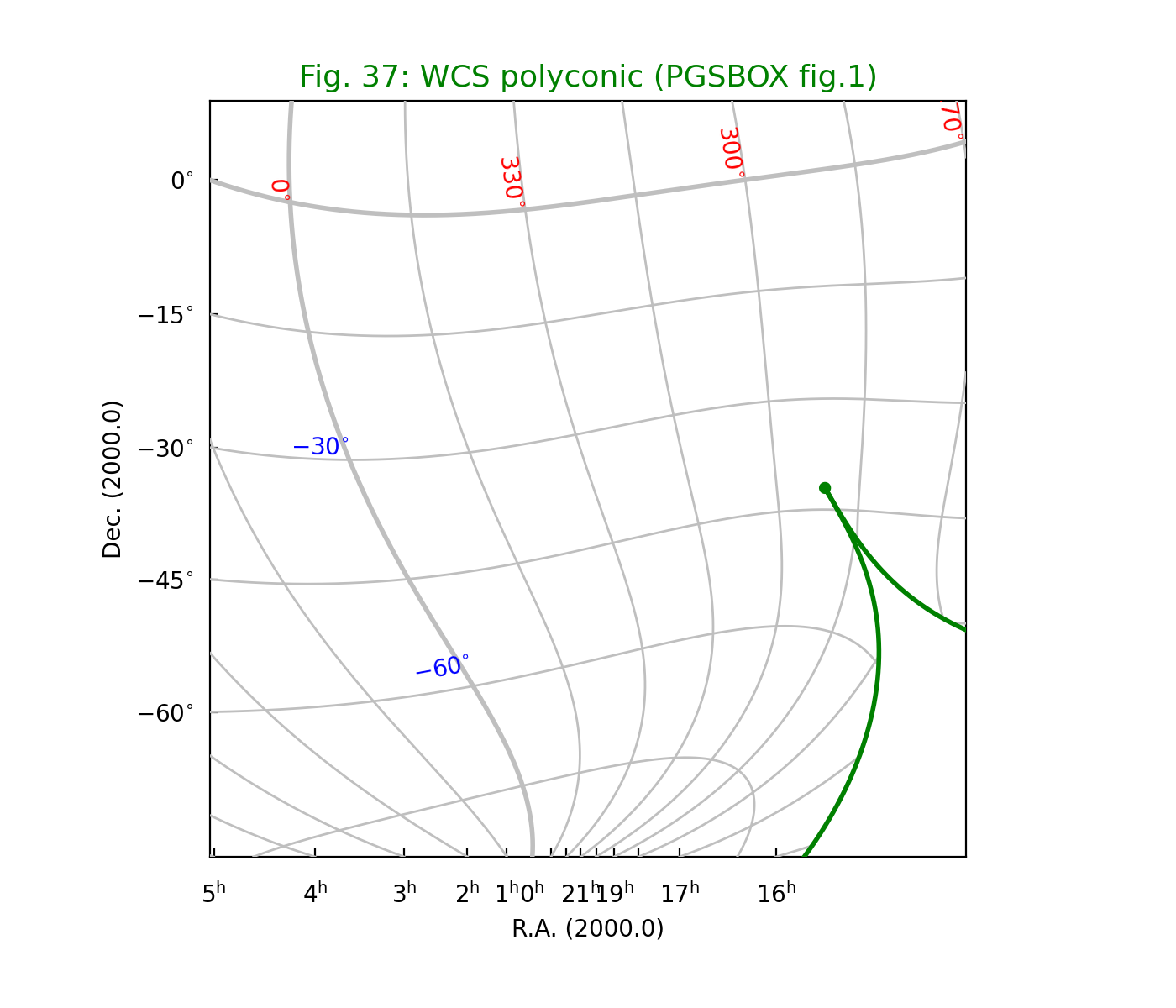
Fig.37: WCS polyconic
Without any tuning, we would observe jumpy behaviour near the dicontinuity of the green border. The two vertical parts would be connected by a small horizontal line. We can improve the plot by increasing the value of parameter gridsamples in the Graticule constructor from 1000 (which is the default value) to 4000. See equivalent plot at http://www.atnf.csiro.au/people/mcalabre/WCS/PGSBOX/index.html
from kapteyn import maputils
import numpy
from service import *

fignum = 37
fig = plt.figure(figsize=figsize)
frame = fig.add_axes((0.1,0.15,0.8,0.75))
title = 'WCS polyconic (PGSBOX fig.1)'
rot = 30.0 *numpy.pi/180.0
header = {'NAXIS'  : 2, 'NAXIS1': 512, 'NAXIS2': 512,
          'CTYPE1' : 'RA---PCO',
          'PC1_1' : numpy.cos(rot), 'PC1_2' : numpy.sin(rot),
          'PC2_1' : -numpy.sin(rot), 'PC2_2' : numpy.cos(rot),
          'CRVAL1' : 332.0, 'CRPIX1' : 192, 'CUNIT1' : 'deg', 'CDELT1' : -1.0/5.0,
          'CTYPE2' : 'DEC--PCO',
          'CRVAL2' : 40.0, 'CRPIX2' : 640, 'CUNIT2' : 'deg', 'CDELT2' : 1.0/5.0,
          'LONPOLE' : -30.0
         }
X = numpy.arange(-180,180.0,15.0);
Y = numpy.arange(-75,90,15.0)
# Here we demonstrate how to avoid a jump at the right corner boundary
# of the plot by increasing the value of 'gridsamples'.
f = maputils.FITSimage(externalheader=header)
annim = f.Annotatedimage(frame)
grat = annim.Graticule(axnum= (1,2), wylim=(-90,90.0), wxlim=(-180,180),
                       startx=X, starty=Y, gridsamples=4000)
grat.setp_lineswcs0(0, lw=2)
grat.setp_lineswcs1(0, lw=2)
grat.setp_tick(wcsaxis=0, position=15*numpy.array((18,20,22,23)), visible=False)
grat.setp_tick(wcsaxis=0, fmt="Hms")
grat.setp_tick(wcsaxis=1, fmt="Dms")
header['CRVAL1'] = 0.0
header['CRVAL2'] = 0.0
header['LONPOLE'] = 999
border = annim.Graticule(header, axnum= (1,2), wylim=(-90,90.0), wxlim=(-180,180),
                         startx=(180-epsilon, -180+epsilon), starty=(-89.5,))
border.setp_gratline((0,1), color='g', lw=2)
border.setp_plotaxis((0,1,2,3), mode='no_ticks', visible=False)
lon_world = list(range(0,360,30))
lat_world = [-dec0, -60, -30, 30, 60, dec0]
labkwargs0 = {'color':'r', 'va':'bottom', 'ha':'right'}
labkwargs1 = {'color':'b', 'va':'bottom', 'ha':'right'}
doplot(frame, fignum, annim, grat, title,
       lon_world=lon_world, lat_world=lat_world,
       labkwargs0=labkwargs0, labkwargs1=labkwargs1)
(Source code, png, hires.png, pdf)
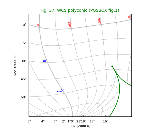
Fig.38: WCS conic equal area projection
See equivalent plot at http://www.atnf.csiro.au/people/mcalabre/WCS/PGSBOX/index.html
from kapteyn import maputils
import numpy
from service import *

fignum = 38
fig = plt.figure(figsize=figsize)
frame = fig.add_axes((0.1,0.1,0.8,0.75))
theta_a = 60.0; eta = 15.0
title = r"""WCS conic equal area projection with
$\theta_a=60^\circ$ and $\eta=15^\circ$ (Cal. PGSBOX fig.2)"""
header = {'NAXIS'  : 2, 'NAXIS1': 512, 'NAXIS2': 512,
          'CTYPE1' : 'RA---COE',
          'CRVAL1' : 90.0, 'CRPIX1' : 256, 'CUNIT1' : 'deg', 'CDELT1' : -1.0/3.0,
          'CTYPE2' : 'DEC--COE',
          'CRVAL2' : 30.0, 'CRPIX2' : 256, 'CUNIT2' : 'deg', 'CDELT2' : 1.0/3.0,
          'LONPOLE' : 150.0,
          'PV2_1'  : theta_a, 'PV2_2' : eta
         }
X = numpy.arange(0,390.0,30.0);
Y = numpy.arange(-60,90,30.0)
f = maputils.FITSimage(externalheader=header)
annim = f.Annotatedimage(frame)
grat = annim.Graticule(axnum= (1,2), wylim=(-90,90.0), wxlim=(0,360),
                       startx=X, starty=Y)
grat.setp_lineswcs0(color='r')
grat.setp_lineswcs1(color='b')
grat.setp_lineswcs0(0, lw=2)
grat.setp_lineswcs1(0, lw=2)
grat.setp_tick(plotaxis=1, position=(150.0,210.0), visible=False)
grat.setp_tick(wcsaxis=0, fmt="Hms")
grat.setp_tick(wcsaxis=1, fmt="Dms")
deltapx = 10
# Draw border with standard graticule
header['CRVAL1'] = 0.0;
header['CRVAL2'] = 60.0
header['LONPOLE'] = 999
header['LATPOLE'] = 999
border = annim.Graticule(header, axnum= (1,2), wylim=(-90,90.0), wxlim=(-180,180),
                         startx=(180-epsilon, -180+epsilon), starty=(-90,90))
border.setp_gratline((0,1), color='g', lw=2)
border.setp_plotaxis((0,1,2,3), mode='no_ticks', visible=False)
framebgcolor = 'k'  # i.e. black
lon_world = list(range(0,360,30))
lat_world = [-dec0, -60, -30, 30, 60, dec0]
labkwargs0 = {'color':'w', 'va':'bottom', 'ha':'right'}
labkwargs1 = {'color':'w', 'va':'bottom', 'ha':'right'}
doplot(frame, fignum, annim, grat, title,
       lon_world=lon_world, lat_world=lat_world,
       labkwargs0=labkwargs0, labkwargs1=labkwargs1,
       framebgcolor=framebgcolor)
(Source code, png, hires.png, pdf)
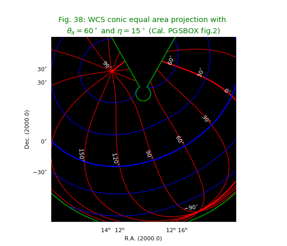
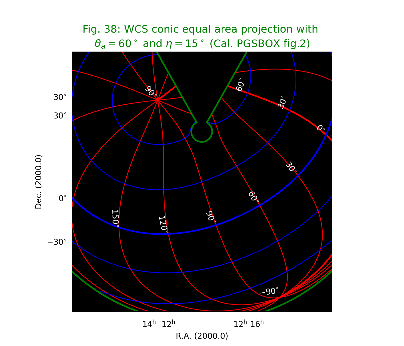

Fig.39: Bonne’s equal area projection (BON) II
See equivalent plot at http://www.atnf.csiro.au/people/mcalabre/WCS/
from kapteyn import maputils
import numpy
from service import *

fignum = 39
fig = plt.figure(figsize=figsize)
frame = fig.add_axes(plotbox)
theta1 = 35
title = r"""Bonne's equal area projection (BON) with conformal latitude
$\theta_1=35^\circ$ and $\alpha_p=0^\circ$, $\theta_p=+45^\circ$ and N.C.P. at $(45^\circ,0^\circ)$.
(Cal. PGSBOX example)"""
header = {'NAXIS'  : 2, 'NAXIS1': 100, 'NAXIS2': 80,
          'CTYPE1' : 'RA---BON',
          'CRVAL1' : 0.0, 'CRPIX1' : 50, 'CUNIT1' : 'deg', 'CDELT1' : -4.0,
          'CTYPE2' : 'DEC--BON',
          'CRVAL2' : 0.0, 'CRPIX2' : 35, 'CUNIT2' : 'deg', 'CDELT2' : 4.0,
          'PV2_1'  : theta1
         }
X = polrange()
Y = numpy.arange(-75.0,90,15.0)
f = maputils.FITSimage(externalheader=header)
annim = f.Annotatedimage(frame)
grat = annim.Graticule(axnum= (1,2), wylim=(-90,90.0), wxlim=(0,360),
                       startx=X, starty=Y)
grat.setp_lineswcs0(color='#339333')  # Dark green
grat.setp_lineswcs1(color='#339333')
header['LONPOLE'] = 45.0  # Or PV1_3
header['CRVAL1'] = 0.0
header['CRVAL2'] = 45.0
oblique = annim.Graticule(header, axnum= (1,2), wylim=(-90,90.0), wxlim=(0,360),
                          startx=X, starty=Y)
oblique.setp_lineswcs0(0.0, color='y')
oblique.setp_lineswcs1(0.0, color='y')
oblique.setp_lineswcs0(list(range(15,360,45)), color='b')
oblique.setp_lineswcs1([15,-15,60, -60], color='b')
oblique.setp_lineswcs0(list(range(30,360,45)), color='r')
oblique.setp_lineswcs1([30,-30,75, -75], color='r')
oblique.setp_lineswcs0(list(range(45,360,45)), color='w')
oblique.setp_lineswcs1((-45,45), color='w')
framebgcolor = 'k'
if not smallversion:
   txt ="""Green:  Native, non-oblique graticule.  Yellow: Equator and prime meridian
Others: Colour coded oblique graticule"""
plt.figtext(0.1, 0.008, txt, fontsize=6)
labkwargs0 = {'visible':False}  # No labels at all!
labkwargs1 = {'visible':False}
doplot(frame, fignum, annim, grat, title,
       labkwargs0=labkwargs0, labkwargs1=labkwargs1,
       framebgcolor=framebgcolor)
(Source code, png, hires.png, pdf)
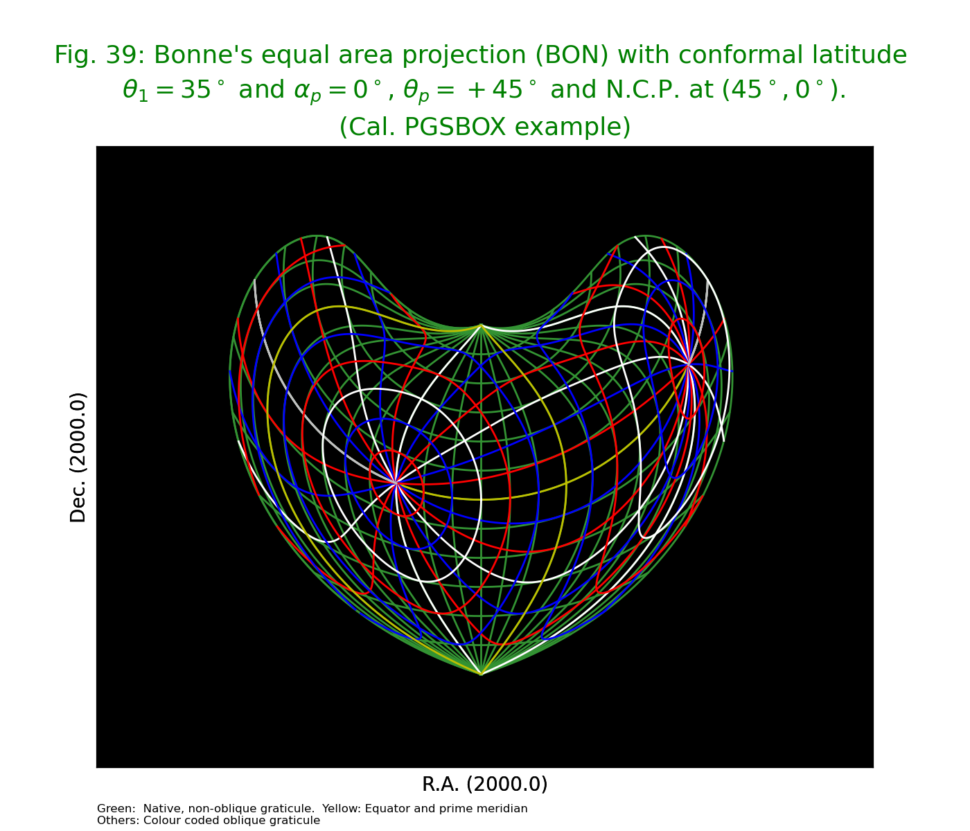
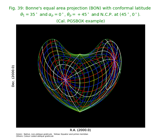
Projection aliases
Table A.1. in [Ref2] lists many alternative projections. These are either one of the projections listed in previous sections or they have special projection parameters. This table lists those parameters and in table 13 of [Ref2] one can find the corresponding PV keyword.
For example if we want a Peter’s projection, then in table A.1. we read that this is in fact a Gall’s orthographic projection (CEA) with \(\lambda = 1/2\). In table 13 we find that for projection CEA the parameter \(\lambda\) corresponds to keyword PVi_1a. This keyword is associated with the latitude axis. If this is the second axis in a FITS header and if we don’t use an alternate header description, then this keyword is PV1_1.
Source code of the service module
from kapteyn import maputils, tabarray
import numpy
import sys
from matplotlib import pyplot as plt


__version__ = '2.0'

epsilon = 0.0000000001

def radians(a):
   return a*numpy.pi/180.0

def degrees(a):
   return a*180.0/numpy.pi

def cylrange():
   X = numpy.arange(0,400.0,30.0);
   # Replace last two (dummy) values by two values around 180 degrees
   X[-1] = 180.0 - epsilon
   X[-2] = 180.0 + epsilon
   return X

def polrange():
   X = numpy.arange(0,380.0,15);
   # Replace last two (dummy) values by two values around 180 degrees
   X[-1] = 180.0 - epsilon
   X[-2] = 180.0 + epsilon
   return X


def getperimeter(grat):
   # Calculate perimeter of QUAD projection
   xlo, y = grat.gmap.topixel((-45.0-epsilon, 0.0))
   xhi, y = grat.gmap.topixel((315+epsilon, 0.0))
   x, ylo = grat.gmap.topixel((180, -45))
   x, yhi = grat.gmap.topixel((180, 45))
   x1, y = grat.gmap.topixel((45-epsilon, 0.0))
   x, ylolo = grat.gmap.topixel((0, -135+epsilon))
   x, yhihi = grat.gmap.topixel((0, 135-epsilon))
   perimeter = [(xlo,ylo), (x1,ylo), (x1,ylolo), (xhi,ylolo), (xhi,yhihi),
                (x1,yhihi), (x1,yhi), (xlo,yhi), (xlo,ylo)]
   return perimeter


def plotcoast(fn, frame, grat, col='k', lim=100, decim=5, plotsym=None, sign=1.0):
   coasts = tabarray.tabarray(fn, comchar='s')  # Read two columns from file
   for segment in coasts.segments:
      coastseg = coasts[segment].T
      xw = sign * coastseg[1]; yw = coastseg[0] # First one appears to be Latitude
      xs = xw; ys = yw                          # Reset lists which store valid pos.
      if 1:
         # Mask arrays if outside plot box
         xp, yp = grat.gmap.topixel((numpy.array(xs),numpy.array(ys)))
         # Be sure you understand
         # the operator precedence: (a > 2) | (a < 5) is the proper syntax
         # because a > 2 | a < 5 will result in an error due to the fact
         # that 2 | a is evaluated first.
         xp = numpy.ma.masked_where(numpy.isnan(xp) |
                              (xp > grat.pxlim[1]) | (xp < grat.pxlim[0]), xp)
         yp = numpy.ma.masked_where(numpy.isnan(yp) |
                              (yp > grat.pylim[1]) | (yp < grat.pylim[0]), yp)
         # Mask array could be of type numpy.bool_ instead of numpy.ndarray
         if numpy.isscalar(xp.mask):
            xp.mask = numpy.array(xp.mask, 'bool')
         if numpy.isscalar(yp.mask):
            yp.mask = numpy.array(yp.mask, 'bool')
         # Count the number of positions in this list that are inside the box
         xdc = []; ydc = []
         for i in range(len(xp)):
            if not xp.mask[i] and not yp.mask[i]:
               if not i%decim:
                  xdc.append(xp.data[i])
                  ydc.append(yp.data[i])
         if len(xdc) >= lim:
            if plotsym == None:
               frame.plot(xdc, ydc, color=col)
            else:
               frame.plot(xdc, ydc, '.', markersize=1, color=col)


# Set defaults which can be overwritten by the allskyfxx.py scripts
title = ''
titlepos = 1.02
dec0 = 89.9999999999
fsize = 10
figsize = (7,6)
drawgrid = False
grat = None
smallversion = False
plotbox = (0.1,0.05,0.8,0.8)
markerpos = "120 deg 60 deg"


def doplot(frame, fignum, annim, grat, title,
           lon_world=None, lat_world=None,
           lon_constval=None, lat_constval=None,
           lon_fmt=None, lat_fmt=None,
           markerpos=None,
           plotdata=False, perimeter=None, drawgrid=None,
           smallversion=False, addangle0=0.0, addangle1=0.0,
           framebgcolor=None, deltapx0=0.0, deltapy0=0.0,
           deltapx1=0.0, deltapy1=0.0,
           labkwargs0={'color':'r'}, labkwargs1={'color':'b'}):
# Apply some extra settings

   if framebgcolor != None:
      frame.set_facecolor(framebgcolor)

   # Plot coastlines if required
   if plotdata:
      if fignum == 36:
         plotcoast('WDB/world.txt', frame, grat, col='k', lim=100)
      else:
         plotcoast('WDB/world.txt', frame, grat, col='r', lim=50,
                    decim=20, plotsym=',', sign=-1)


   if lon_constval == None:
      lon_constval = 0.0    # Reasonable for all sky plots
   if lat_constval == None:
      lat_constval = 0.0    # Reasonable for all sky plots
   if lon_fmt == None:
      lon_fmt = 'Dms'
   if lat_fmt == None:
      lat_fmt = 'Dms'
   # Plot labels inside graticule if required
   #labkwargs0.update({'fontsize':fsize})
   #labkwargs1.update({'fontsize':fsize})
   ilabs1 = grat.Insidelabels(wcsaxis=0,
                        world=lon_world, constval=lat_constval,
                        deltapx=deltapx0, deltapy=deltapy0,
                        addangle=addangle0, fmt=lon_fmt, **labkwargs0)
   ilabs2 = grat.Insidelabels(wcsaxis=1,
                        world=lat_world, constval=lon_constval,
                        deltapx=deltapx1, deltapy=deltapy1,
                        addangle=addangle1, fmt=lat_fmt, **labkwargs1)

   # Plot just 1 pixel c.q. marker
   if markerpos != None:
      annim.Marker(pos=markerpos, marker='o', color='red')

   if drawgrid:
      pixellabels = annim.Pixellabels(plotaxis=(2,3))

   # Plot the title
   title = "Fig. %d: "%fignum + title
   if smallversion:
      t = frame.set_title(title, color='g', fontsize=10)
   else:
      t = frame.set_title(title, color='g', fontsize=13, linespacing=1.5)
   t.set_y(titlepos)
   annim.plot()

   # Plot alternative borders. Do this after the graticule is plotted
   # Only then you know the frame of the graticule and plotting in that
   # frame will overwrite graticule lines so that the borders look better
   if perimeter != None:
      p = plt.Polygon(perimeter, facecolor='#d6eaef', lw=2)
      frame.add_patch(p)     # Must be in frame specified by user
      Xp, Yp = list(zip(*perimeter))
      grat.frame.plot(Xp, Yp, color='r')

   annim.interact_toolbarinfo()

   plt.show()