Voronoi Patterns & Geometric Scaling
 Appendix to referee report
Revs. Mod. Phys. (Jones et al., 2003)
Appendix to referee report
Revs. Mod. Phys. (Jones et al., 2003)
Appendix to referee report
Revs. Mod. Phys. (Jones et al., 2003)
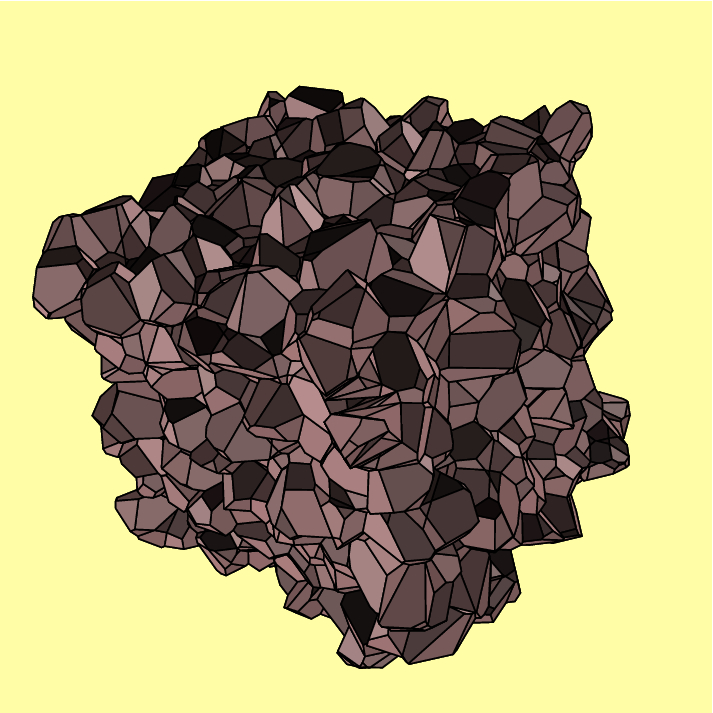
Figure 1. A 3-D Voronoi tessellation of 1000 cells
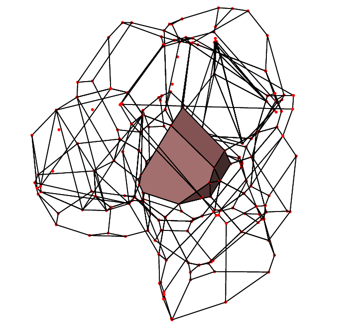
Figure 2. Wire diagram view of Voronoi cells,
edges indicated by solid lines, vertices by red dots
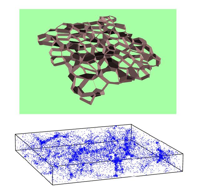
Figure 3. Slices through 3-D Voronoi tessellation:
top: geometric view
bottom: slice through Voronoi kinematic model particle distribution
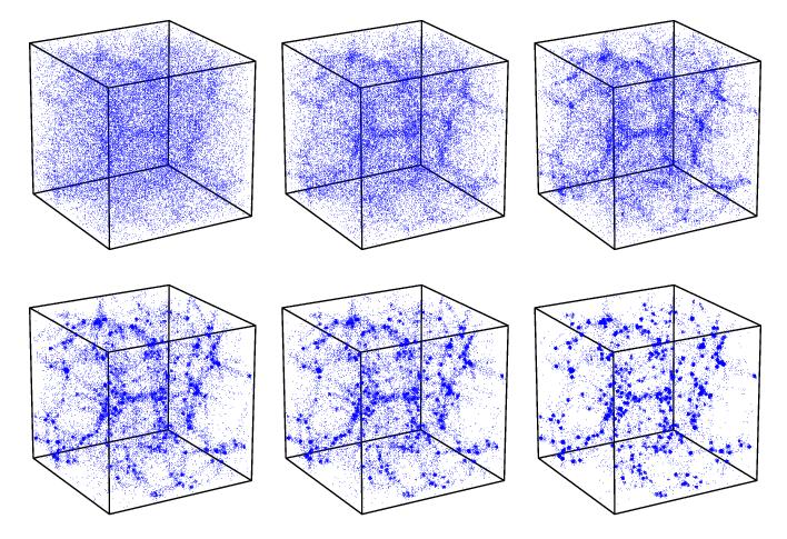
Figure 4. Evolution Voronoi kinematic model
particle distribution in Voronoi kinematic model at 6 successive timesteps
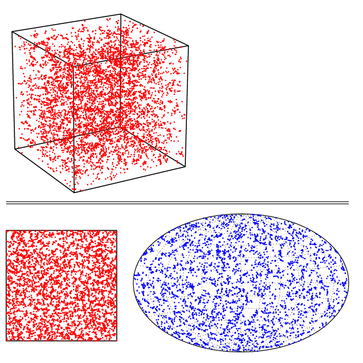
Figure 5. Voronoi vertex distribution
top: spatial distribution
bottom left: slice through 3-D distribution
bottom right: Aitoff projection of vertex sky distribution
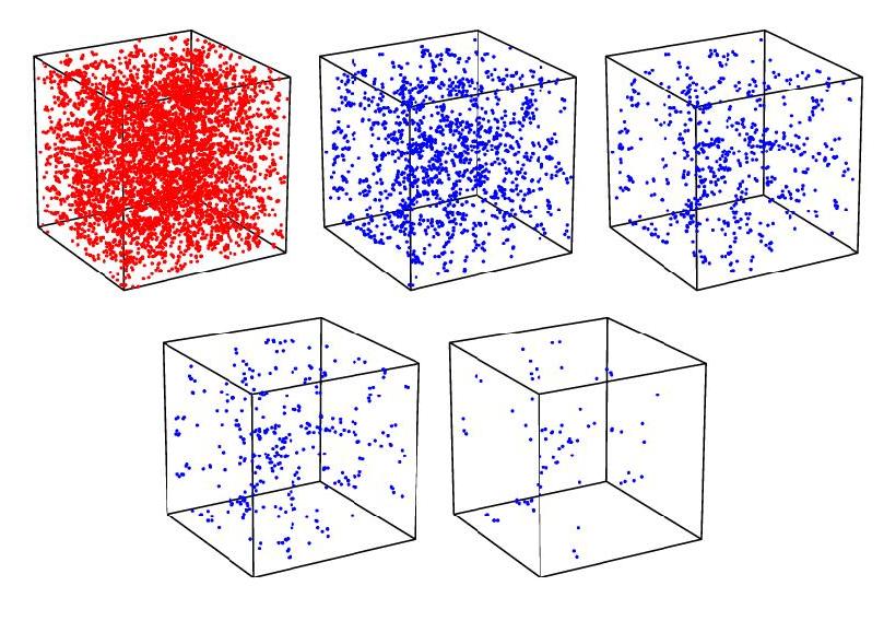
Figure 6. Voronoi vertex distribution bias:
spatial Voronoi vertex distribution for vertex samples,
selected at 5 successively richer "vertex mass" limits
(top left --> bottom right: complete sample, 25%, 12.5%, 5%, 1% richest
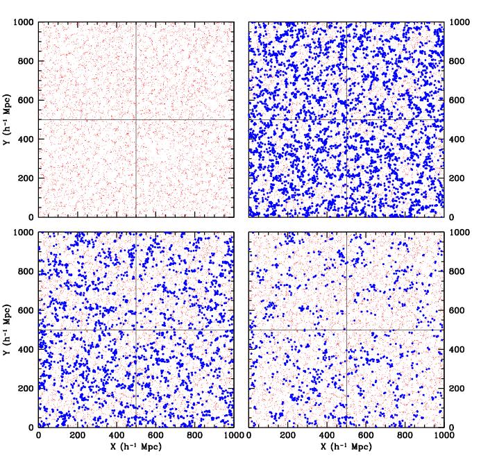
Figure 7. Voronoi vertex distribution bias:
Voronoi vertex distribution in central slice. Red dots: complete sample of Voronoi vertices
In three successive frames (top right, bottom left, bottom right) blue dots indicate
samples of 25%, 12.5% and 5% richest vertices
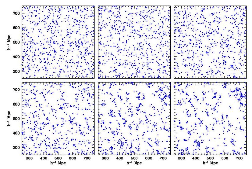
Figure 8. Voronoi vertex distribution bias:
6 samples of Voronoi vertices for 6 successive richnesses
(top left --> bottom right: full sample to 1% richest), scaled to equal number density.
Clear demonstration that differences in distribution not only due to number density but
also to differences in clustering properties
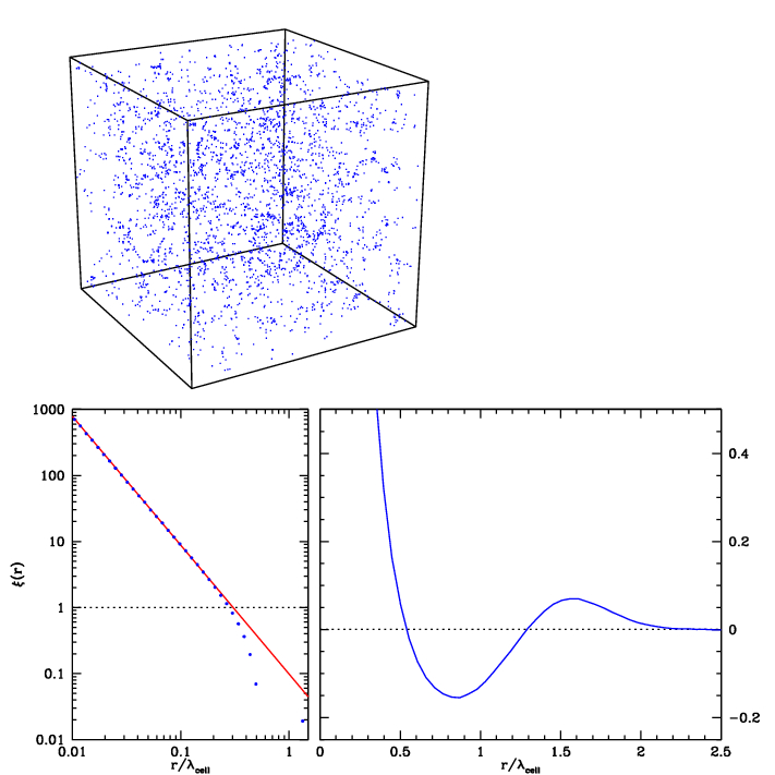
Figure 9. Voronoi vertex clustering
Two-point correlation function full Voronoi sample
top: spatial Voronoi vertex sample
bottom left: log-log plot xi(r); bottom right: lin-lin plot xi(r)
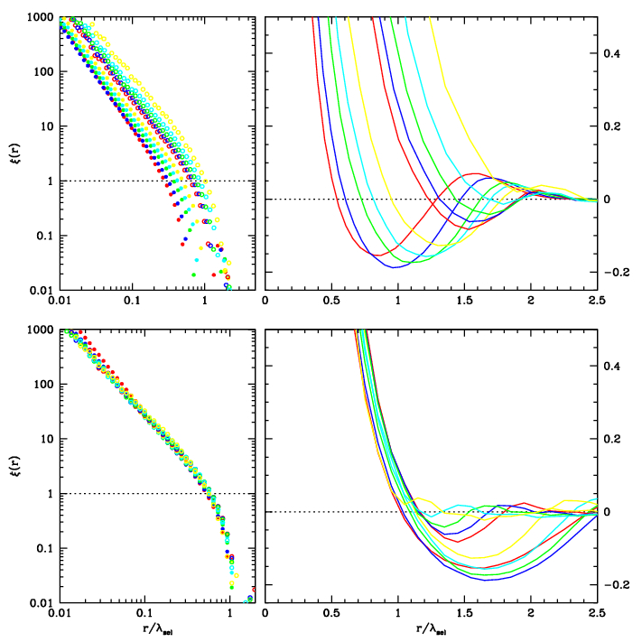
Figure 10. Voronoi vertex clustering
Two-point correlation function for samples of Voronoi vertices, a sequence of 10 samples of
successively richer (more massive) vertices:
top: log-log and lin-lin plots two-point correlation function, as function of true distance
bottom: same, but distance scaled to inter-vertex distance in samples
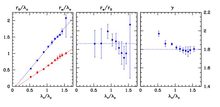
Figure 11. Voronoi vertex clustering: Geometric selfsimilarity ?
left: scaling of clustering length r_0 (xi(r_0)=1) and
correlation length r_a (spatial coherence length at which xi(r_a)=0),
as function of inter-vertex distance lambda_v (lambda_c is basic distance unit,
here equal to distance between tessellation nuclei)
centre: scaling ratio correlation length r_a/clustering length r_0 as
function inter-vertex distance lambda_v:
constant ratio indicates self-similarity Voronoi vertex scaling
right: scaling power-law index gamma of power-law regime correlation function xi(r)
as function of inter-vertex distance lambda_v
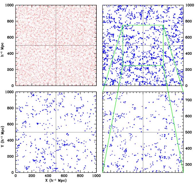
Figure 12. Significance geometric selfsimilarity:
Top left: slice through full sample Voronoi vertices (red dots)
Top right: selected 25% richest vertices from full sample,
green box: central box of 1/8 volume complete box
Bottom left: select 3.125% richest vertices from full sample,
Bottom right: vertex distribution green box inflated to same size, this scaling
yields spatial point distribution similar to that of 3.125% richest vertices