Background information spectral translations
Introduction
This background information has been written for two reasons. First we wanted to get
some understanding of the conversions between spectral quantities and second,
we wanted to have some knowledge about legacy FITS headers (of which there must be
a lot) where applying the conversions of WCSLIB in the context of module wcs
without modifications will give wrong results.
Warning
One needs to be aware of the fact that WCSLIB converts between frequencies and velocities in the same reference system while in legacy FITS headers it is common to give a topocentric reference frequency and a reference velocity in a different reference system.
Alternate headers for a spectral line example
In “Representations of spectral coordinates in FITS” ([Ref3] ), section 10.1 deals with an example of a VLA spectral line cube which is regularly sampled in frequency (CTYPE3=’FREQ’). The section describes how one can define alternative FITS headers to deal with different velocity definitions. We want to examine this exercise in more detail than provided in the article to illustrate how a FITS header can be modified and serve as an alternate header.
The topocentric spectral properties in the FITS header from the paper are:
CTYPE3= 'FREQ'
CRVAL3=  1.37835117405e9
CDELT3=  9.765625e4
CRPIX3=  32
CUNIT3= 'Hz'
RESTFRQ= 1.420405752e+9
SPECSYS='TOPOCENT'
Note
For a pixel coordinate \(N\), reference pixel \(N_{ref}\) with reference world coordinate \(W_{ref}\) and a step size in world coordinates \(\Delta W\), the world coordinate \(W\) is calculated with:
If CTYPE contains a code for a non linear conversion algorithm (as in CTYPE=’VOPT-F2W’) then this relation cannot be applied.
As stated in the note above, code for a conversion algorithm is important. The statements can be verified with the following script:
#!/usr/bin/env python
from kapteyn import wcs

Z0 = 9120000              # Barycentric optical reference velocity
dZ0 = -2.1882651e+4       # Increment in barycentric optical velocity
N = 32                    # Pixel coordinate of reference pixel

header = {  'NAXIS'   :  1,
            'RESTWAV' :  0.211061140507,   # [m]
            'CTYPE1'  : 'VOPT',
            'CRVAL1'  :  Z0,               # [m/s]
            'CDELT1'  :  dZ0,              # [m/s]
            'CRPIX1'  :  N,
            'CUNIT1'  : 'm/s'
         }
spec = wcs.Projection(header)
print "From VOPT: Pixel, velocity wcs, velocity linear (%s)" % spec.units
pixels = range(30,35)
Vwcs = spec.toworld1d(pixels)
for p,v in zip(pixels, Vwcs):
   print p, v/1000.0, (Z0 + (p-N)*dZ0)/1000.0

header = {  'NAXIS'   :  1,
            'CNAME1'  : 'Barycentric optical velocity',
            'RESTWAV' :  0.211061140507,   # [m]
            'CTYPE1'  : 'VOPT-F2W',
            'CRVAL1'  :  Z0,               # [m/s]
            'CDELT1'  :  dZ0,              # [m/s]
            'CRPIX1'  :  N,
            'CUNIT1'  : 'm/s'
         }
spec = wcs.Projection(header)
print "From VOPT-F2W: Pixel, velocity wcs, velocity linear (%s)" % spec.units
pixels = range(30,35)
Vwcs = spec.toworld1d(pixels)
for p,v in zip(pixels, Vwcs):
   print p, v/1000.0, (Z0 + (p-N)*dZ0)/1000.0

# Output:
#
# From VOPT: Pixel, velocity wcs, velocity linear (m/s)
# Conversion is linear; no differences
# 30 9163.765302 9163.765302
# 31 9141.882651 9141.882651
# 32 9120.0 9120.0
# 33 9098.117349 9098.117349
# 34 9076.234698 9076.234698
# From VOPT-F2W: Pixel, velocity wcs, velocity linear (m/s)
# Conversion is not linear
# 30 9163.77150335 9163.765302
# 31 9141.88420123 9141.882651
# 32 9120.0 9120.0
# 33 9098.11889901 9098.117349
# 34 9076.24089759 9076.234698
Relation optical velocity and barycentric/lsrk reference frequency
Let’s start to find the alternate header information for the header from article in [Ref3] . The extra information about the velocity there is that we have an optical barycentric velocity of 9120 km/s (as required by an observer) stored as an alternate FITS keyword CRVAL3Z.:
CTYPE3Z= 'VOPT-F2W'
CRVAL3Z=  9.120e+6      / [m/s]
The relation between frequency and optical velocity requires a rest frequency (RESTFRQ=). The relation is:
We adopted variable Z for velocities following the optical definition. The header tells us that equal steps in pixel coordinates are equal steps in frequency and the formula above shows that these steps in terms of optical velocity depends on the frequency in a non-linear way. Therefore we set the conversion algorithm to F2W which indicates that there is a non linear conversion from frequency to wavelength (optical velocities are associated with wavelength, see [Ref3] .). Note that we can use wildcards for the non linear conversion algorithm, so CTYPE3Z=’VOPT-???’ is also allowed in our programs.
We can rewrite equation 1 into:
If we enter the numbers we get a barycentric HI reference frequency:
and we have part of a new alternate header:
CTYPE3F= 'FREQ'
CRVAL3F= 1.37847121643e+9 / [Hz]
So given an optical velocity in a reference system (in our case the barycentric system), we can calculate which barycentric frequency we can use as a reference frequency. For a conversion between a barycentric frequency and a barycentric velocity we also need to know what the barycentric frequency increment is.
Barycentric/lsrk frequency increments
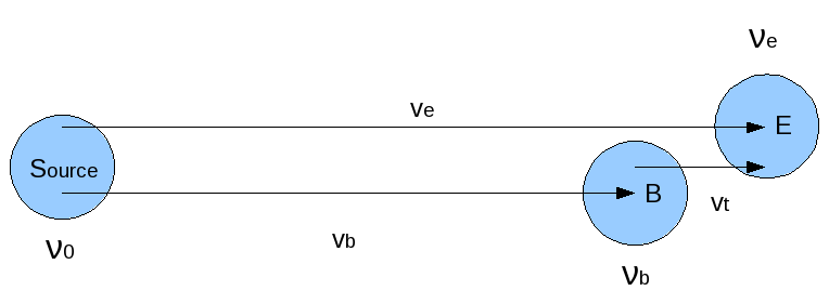
fig.1 Overview of velocities and frequencies of barycenter (B) and Earth (E) w.r.t. source. The arrows represent velocities. The object and the Earth are moving. The longest arrow represents the (relativistic) addition of two velocities
Let’s use index b for variables bound to the barycentric system and e for the topocentric system. This frequency, \(\nu_b\) =1.37847121643 GHz is greater than the reference frequency \(\nu_e\) at the observatory (FITS keyword CRVAL3= 1.37835117405 GHz).
The difference between frequencies in the topocentric and barycentric system is caused by the difference between the velocities of reference frames B and E at the time of observation.
This velocity is a true velocity. It is called the topocentric correction.
Let’s try to find an expression for this topocentric correction in terms of frequencies. The relation between a true velocity and a shift in frequency is given by the formula
If we want to express the apparent radial velocity in terms of frequencies, then this can be written as:
For the apparent radial velocities \(v_b\) and \(v_e\) we have:
and:
The relativistic addition of velocities in fig. 1. requires:
which gives the topocentric correction as:
With the numbers inserted we find:
If the FITS header has keywords with the position of the source, the time of observation and the location of the observatory then one can calculate the topocentric correction by hand. This information was needed at the observatory to set a frequency for a given barycentric velocity. However many FITS files do not have enough information to calculate the topocentric correction. Also it is not needed if one knows the shifted frequencies \(\nu_e\) and \(\nu_b\) , then we can calculate the topocentric velocity without calculating the apparent radial velocities. This can be shown if we insert the expressions for velocities \(v_e\) and \(v_b\) in the expression for \(v_t\) . Then after some rearranging one finds:
and with the numbers:
which is consistent with (11).
VELOSYSZ=26108 / [m/s]
With a given topocentric correction and the reference frequency in the barycenter we can reconstruct the reference frequency at the observatory with (12) written as:
Note
1) It is important to realize that the reference frequency at E is smaller than the reference frequency at B because w.r.t. the source E moves faster than B. So if there is a change in the velocity of the source, the frequencies in B and E will change, but the topocentric correction keeps the same value and therefore the relation between the frequencies \(\nu_e\) and \(\nu_b\) remains the same (eq. (14)).
Note
2) If we forget about the source and we have an event on E with a certain frequency then an observer in barycenter B will observe a lower frequency. This is because on the line that connects the source and B, the observatory at E moves away from B which decreases the remote frequency.
So if we change a frequency on E by tuning the receiver at the observatory at frequency \(\nu_e + \Delta \nu_e\) , then the observer at B would observe a smaller frequency \(\nu_b + \Delta \nu_b\) . The amount of the decrease is related to the topocentric correction as follows:
and therefore we can write for the frequency bandwidth in B:
At first it seems that this contradicts eq. (14) (where the indices seem to be swapped), but this is not true because we changed the frame of the observer from Earth to the barycenter. The event was in E and it is observed in B.
The increment in frequency therefore becomes 97.64775 kHz:
CDELT3F= 9.764775e+4 / [Hz]
So if we change CRVAL1 and CDELT1 in our demonstration script to the barycentric values, we get the barycentric optical convention velocities for the pixels. As a check we listed the script and the value for pixel 32 which is exactly 9120 (km/s):
#!/usr/bin/env python
from kapteyn import wcs
header  = { 'NAXIS'  : 1,
            'CTYPE1' : 'FREQ',
            'CRVAL1' : 1378471216.4292786,
            'CRPIX1' : 32,
            'CUNIT1' : 'Hz',
            'CDELT1' : 97647.745732,
            'RESTFRQ': 1.420405752e+9
         }
spec = wcs.Projection(header).spectra('VOPT-F2W')
pixels = range(30,35)
Vwcs = spec.toworld1d(pixels)
print "Pixel, velocity (%s)" % spec.units
for p,v in zip(pixels, Vwcs):
   print p, v/1000.0

print "Pixel at velocity 9120 km/s: ", spec.topixel1d(9120000)
# Output
# Pixel, velocity (m/s)
# 30 9163.77150423
# 31 9141.88420167
# 32 9120.0
# 33 9098.11889856
# 34 9076.2408967
# Pixel at velocity 9120 km/s:  32.0
Note: A closure test is added with method topixel1d()
Note
In the previous two sections we started with a topocentric frequency and a topocentric frequency increment and derived values for a barycentric frequency and a barycentric frequency increment. These values can be used to set an alternate header (barycentric frequency system ‘F’) for which we can convert between frequency and optical velocity. For GIPSY legacy headers these steps are used to convert between topocentric frequencies and velocities in another reference system, See A recipe for modification of Nmap/GIPSY FITS data
Increment in barycentric/lsrk optical velocity
The optical velocity was given by:
Its derivative is:
But for \(\nu\) we have the expression:
so we end up with:
With \(d\nu = \Delta \nu_b\) and the given barycentric velocity \(Z_b\) = 9120000 m/s, this gives an increment in optical velocity of:
With these values we explained some other alternate header keywords in the basic spectral-line example:
CDELT3Z= -2.1882651e+4  / [m/s]
SPECSYSZ= 'BARYCENT'    / Velocities w.r.t. barycenter
SSYSOBSZ= 'TOPOCENT'    / Observation was made from the 'TOPOCENT' frame
Barycentric/lsrk radio velocity
For radio velocities one needs to apply the definition:
and for the shifted frequency we derive from this equation:
and the spectral translation code becomes: proj.spectra(‘VRAD’)
In the next code example we demonstrate for a barycentric radio velocity V = 8850.750904 km/s how to calculate the barycentric velocities at arbitrary pixels. This velocity is derived from the optical example in a way that shifted frequency and topocentric correction are the same. One can use the formula
to find the value of \(V_b = 1.37847121643*9120/1.420405752 = 8850.750904\) km/s (with the frequencies in GHz and the velocity in km/s). In a next section we will derive this value in another way; see (26) and (27)
#!/usr/bin/env python
from kapteyn import wcs
import numpy as n

c = 299792458.0       # Speed of light (m/s)
f = 1.37835117405e9   # Topocentric reference frequency (Hz)
df = 9.765625e4       # Topocentric frequency increment (Hz)
f0 = 1.420405752e+9   # Rest frequency (Hz)
V = 8850750.904       # Barycentric radio velocity (m/s)

fb = f0*(1-V/c)
print "Barycentric freq.: ", fb
v = c * ((fb*fb-f*f)/(fb*fb+f*f))
print "VELOSYSR= Topocentric correction:", v, "m/s"
dfb = df*(c-v)/n.sqrt(c*c-v*v)
print "CDELT3F= Delta in frequency in the barycentric frame eq.4): ", dfb

header = { 'NAXIS'  : 1,
           'CTYPE1' : 'FREQ',
           'CRVAL1' : fb,
           'CRPIX1' : 32,
           'CUNIT1' : 'Hz',
           'CDELT1' : dfb,
           'RESTFRQ': 1.420405752e+9
      }
line = wcs.Projection(header).spectra('VRAD')
pixels =  range(30,35)
Vwcs = line.toworld1d(pixels)
for p,v in zip(pixels, Vwcs):
   print p, v/1000

# Output:
# Barycentric freq.:  1378471216.43
# VELOSYSR= Topocentric correction: 26108.1745986 m/s
# CDELT3F= Delta in frequency in the barycentric frame eq.4):  97647.745732
#
# Output Radio velocities (km/s)
# 30 8891.97019316
# 31 8871.36054858
# 32 8850.750904
# 33 8830.14125942
# 34 8809.53161484
Frequency to Radio velocity
From the definition of radio velocity:
we can find a radio velocity that corresponds to the value of the optical velocity. This (barycentric) optical velocity (9120 Km/s) caused a shift of the rest frequency. The new frequency became \(\nu_b = 1.37847122 \times 10^9 Hz\). If we insert this number in the equation above we find:
The formula for a direct conversion from optical to radio velocity can be derived by inserting the formula for the frequency shift corresponding to optical velocity, into the expression for the radio velocity:
With eq. (26) it is easy to find the increment of the velocity if the increment in frequency at the reference frequency is given:
Note that this increment in frequency is the increment in the barycentric system!
Inserting the numbers with \(d\nu = \Delta \nu_b\) we find:
This gives us another two values for the alternate header keywords:
CTYPE3R= 'VRAD'
CRVAL3R= 8.85075090419e+6  / [m/s]
CDELT3R= -2.0609645e+4     / [m/s]
Note that CTYPE3R= ‘VRAD’ indicates that the conversion between frequency and radio velocity is linear.
The next script shows how we can use these new header values to get a list of radio velocities as function of pixel. We commented out the rest frequency. Its value is not necessary because we can rewrite the formulas for the velocity in terms of \(\nu/\nu_0\) and \(\Delta \nu/\nu_0\)
#!/usr/bin/env python
from kapteyn import wcs
header = { 'NAXIS'  : 1,
           'CTYPE1' : 'VRAD',
           'CRVAL1' : 8850750.904193053,
           'CRPIX1' : 32,
           'CUNIT1' : 'm/s',
           'CDELT1' : -20609.644582145629,
#          'RESTFRQ': 1.420405752e+9
         }
line = wcs.Projection(header)
pixels =  range(30,35)
Vwcs = line.toworld1d(pixels)
for p,v in zip(pixels, Vwcs):
   print p, v/1000
#
# Output barycentric radio velocity in km/s:
# 30 8891.97019336
# 31 8871.36054878
# 32 8850.75090419
# 33 8830.14125961
# 34 8809.53161503
Alternatively use the spectral translation method spectra() with the values of the barycentric frequency and frequency increment as follows to get (exactly) the same output:
#!/usr/bin/env python
from kapteyn import wcs
header = { 'NAXIS'  : 1,
           'CTYPE1' : 'FREQ',
           'CRVAL1' : 1378471216.4292786,
           'CRPIX1' : 32,
           'CUNIT1' : 'Hz',
           'CDELT1' : 97647.745732,
           'RESTFRQ': 1.420405752e+9
         }
line = wcs.Projection(header).spectra('VRAD')
pixels =  range(30,35)
Vwcs = line.toworld1d(pixels)
for p,v in zip(pixels, Vwcs):
   print p, v/1000
#
# Output barycentric radio velocity in km/s:
# 30 8891.97019336
# 31 8871.36054878
# 32 8850.75090419
# 33 8830.14125961
# 34 8809.53161503
Frequency to Apparent radial velocity
As written before, the relation between a true velocity and a shifted frequency is:
Observed from the barycenter the source has an apparent radial velocity:
CTYPE3V= 'VELO-F2V'
CRVAL3V= 8.98134229811e+6 / [m/s]
Note that CTYPE3V= ‘VELO-F2V’ indicates that we derived these velocities from a system in which the frequency is linear with the pixel value.
For the increment of the apparent radial velocity we need to find the derivative of eq. (6)
This works out as:
and with the appropriate numbers inserted for \(d\nu = \Delta \nu_b\)
and \(\nu = \nu_b\):
which reveals the value of another keyword from the header in the article’s example:
CDELT3V= -2.1217551e+4 / [m/s]
Sometimes you might encounter an alternative formula that doesn’t list the frequency. It uses eq. (5) to express the frequency in terms of the apparent radial velocity and the rest frequency.
If you insert this into:
then after some rearrangements you end up with the expression:
If you insert v = 8981342.29811 (m/s) in this expression you will get exactly the same apparent radial velocity increment (-2.1217551e+4 m/s).
We found an apparent radial velocity and calculated the increment for this radial velocity. With a short script and a minimal header we demonstrate how to use WCSLIB to get an apparent radial velocity for an arbitrary pixel:
#!/usr/bin/env python
from kapteyn import wcs

header = { 'NAXIS'  : 1,
           'CTYPE1' : 'VELO-F2V',
           'CRVAL1' : 8981342.2981121931,
           'CRPIX1' : 32,
           'CUNIT1' : 'm/s',
           'CDELT1' : -21217.5513673598,
           'RESTFRQ': 1.420405752e+9
         }
line = wcs.Projection(header)
pixels = range(30,35)
Vwcs = line.toworld1d(pixels)
for p,v in zip(pixels, Vwcs):
   print p, v/1000
# Output:
# 30 9023.78022672
# 31 9002.56055595
# 32 8981.34229811
# 33 8960.12545322
# 34 8938.9100213
How can this work? From eq. (36) and eq. (37) it is obvious that WCSLIB can calculate the reference frequency from the reference apparent radial velocity. For this reference frequency and the increment in apparent radial velocity it can calculate the increment in frequency at this reference frequency. Then we have all the information to use eq. (36) to calculate radial velocities for different frequencies (i.e. different pixels). Note that the step in frequency is linear and the step in radial velocity is not (which explains the extension ‘F2V’ in the CTYPE keyword).
Next script and header is an alternative to get exactly the same results. The header lists the barycentric frequency and frequency increment. We need a spectral translation with method spectra() to tell WCSLIB to calculate apparent radial velocities:
#!/usr/bin/env python
from kapteyn import wcs
header  = { 'NAXIS'  : 1,
            'CTYPE1' : 'FREQ',
            'CRVAL1' : 1378471216.4292786,
            'CRPIX1' : 32,
            'CUNIT1' : 'Hz',
            'CDELT1' : 97647.745732,
            'RESTFRQ': 1.420405752e+9
         }
line = wcs.Projection(header).spectra('VELO-F2V')
pixels = range(30,35)
Vwcs = line.toworld1d(pixels)
for p,v in zip(pixels, Vwcs):
   print p, v/1000
# Output:
# 30 9023.78022672
# 31 9002.56055595
# 32 8981.34229811
# 33 8960.12545322
# 34 8938.9100213
Frequency to Wavelength
The rest wavelength is given by the relation:
Inserting the right numbers we find:
For the barycentric wavelength we need to insert the barycentric frequency.
The increment in wavelength as function of the increment in (barycentric) frequency is:
With the right numbers:
This gives us the alternate header keywords:
RESTWAVZ= 0.211061140507 / [m]
CTYPE3W= 'WAVE-F2W'
CRVAL3W=  0.217481841062  / [m]
CDELT3W= -1.5405916e-05   / [m]
CUNIT3W=  'm'
RESTWAVW= 0.211061140507  / [m]
Note that CTYPE indicates that there is a non linear conversion from frequency to wavelength.
From the standard definition of optical velocity:
it follows that the increment in optical velocity as function of increment of wavelength is given by:
Then with the numbers we find:
which is the increment in optical velocity earlier given for CDELT3Z.
This is one of the possible conversions between wavelength and velocity. Others are listed in scs.pdf table 3 of E.W. Greisen et al. page 750.
Conclusions
Note that the inertial system is set by a (FITS) header using a special keyword (e.g. VELREF=) or it is coded in the CTYPEn keyword. It doesn’t change anything in the calculations above. Conversions between inertial reference systems is not possible because headers do (usually) not contain the relevant information to calculate the topocentric correction w.r.t. that system (one needs time of observation, position of observatory and position of the observed source).
From a header with CTYPEn=’FREQ’ we can derive optical, radio and apparent radial velocities with method spectra():
proj = wcs.Projection(header).spectra(‘VOPT-F2W’)
proj = wcs.Projection(header).spectra(‘VRAD’)
proj = wcs.Projection(header).spectra(‘VELO-F2V’)
This applies also to alternate axis descriptions. So if CTYPE1=’VRAD’ one can derive one of the other velocity definitions by adding the spectra() method with the appropriate argument.
Here is an example:
#!/usr/bin/env python
from kapteyn import wcs
wcs.debug = True
header = { 'NAXIS'  : 1,
         'CTYPE1' : 'VRAD',
         'CRVAL1' : 8850750.904193053,
         'CRPIX1' : 32,
         'CUNIT1' : 'm/s',
         'CDELT1' : -20609.644582145629,
         'RESTFRQ': 1.420405752e+9
         }
line = wcs.Projection(header).spectra('VOPT-F2W')
pixels = range(30,35)
Vwcs = line.toworld1d(pixels)
for p,v in zip(pixels, Vwcs):
   print p, v/1000
# Output:
# Velocities in km/s converted from 'VRAD' to 'VOPT-F2W'
# 30 9163.77150423
# 31 9141.88420167
# 32 9120.0
# 33 9098.11889856
# 34 9076.2408967
Note that the rest frequency is required now.
Note also that we added statement wcs.debug = True to get some debug information from WCSLIB.
Axis types ‘FREQ-HEL’ and ‘FREQ-LSR’ (AIPS definitions) are recognized by WCSLIB and are treated as ‘FREQ’. No conversions are done. Internally the keyword SPECSYS= gets a value.
The complete alternate axis descriptions
In this section we summarize the alternate axis descriptions and we add a small script that proves that these descriptions are consistent:
CNAME=  'Topocentric Frequency. Basic header'
CTYPE3= 'FREQ'
CRVAL3=  1.37835117405e9
CDELT3=  9.765625e4
CRPIX3=  32
CUNIT3= 'Hz'
RESTFRQ= 1.420405752e+9
SPECSYS='TOPOCENT'

CNAME3Z= 'Barycentric optical velocity'
RESTWAVZ= 0.211061140507   / [m]
CTYPE3Z= 'VOPT-F2W'
CRVAL3Z=  9.120e+6         / [m/s]
CDELT3Z= -2.1882651e+4     / [m/s]
CRPIX3Z=  32
CUNIT3Z= 'm/s'
SPECSYSZ='BARYCENT'        / Velocities w.r.t. barycenter
SSYSOBSZ='TOPOCENT'        / Observation was made from the 'TOPOCENT' frame
VELOSYSZ= 26108            / [m/s]

CNAME3F= 'Barycentric frequency'
CTYPE3F= 'FREQ'
CRVAL3F=  1.37847121643e+9 / [Hz]
CDELT3F=  9.764775e+4      / [Hz]
CRPIX3F=  32
CUNIT3F= 'Hz'
RESTFRQF= 1.420405752e+9
SPECSYSF='BARYCENT'
SSYSOBSF='TOPOCENT'
VELOSYSF= 26108            / [m/s]

CNAME3R= 'Barycentric radio velocity'
CTYPE3R= 'VRAD'
CRVAL3R=  8.85075090419e+6 / [m/s]
CDELT3R= -2.0609645e+4     / [m/s]
CRPIX3R=  32
CUNIT3R= 'm/s'
RESTFRQR= 1.420405752e+9
SPECSYSR='BARYCENT'
SSYSOBSR='TOPOCENT'
VELOSYSR= 26108            / [m/s]

CNAME3V= 'Barycentric apparent radial velocity'
RESTFRQV= 1.420405752e+9   / [Hz]
CTYPE3V= 'VELO-F2V'
CRVAL3V=  8.98134229811e+6 / [m/s]
CDELT3V= -2.1217551e+4     / [m/s]
CRPIX3V=  32
CUNIT3V= 'm/s'
SPECSYSV='BARYCENT'
SSYSOBSV='TOPOCENT'
VELOSYSV= 26108            / [m/s]

CNAME3W= 'Barycentric wavelength'
CTYPE3W= 'WAVE-F2W'
CRVAL3W=  0.217481841062   / [m]
CDELT3W= -1.5405916e-05    / [m]
CRPIX3W=  32
CUNIT3W= 'm'
RESTWAVW=  0.211061140507  / [m]
SPECSYSW='BARYCENT'
SSYSOBSW='TOPOCENT'
VELOSYSW= 26108            / [m/s]
To check the validity and completeness of these alternate axis descriptions, we wrote a small script that loops over all the mnemonic letter codes in a header that is composed from the header fragments above. We only changed axisnumber 3 to 1. The output is the same within the boundaries of the given precision of the numbers. To change the axis description in a header we use the alter parameter when we create the projection object.
Parameter alter is an optional letter from ‘A’ through ‘Z’, indicating an alternative WCS axis description:
#!/usr/bin/env python
from kapteyn import wcs
header = {  'NAXIS'    :  1,
            'CTYPE1'   : 'FREQ',
            'CRVAL1'   :  1378471216.4292786,
            'CRPIX1'   :  32,
            'CUNIT1'   : 'Hz',
            'CDELT1'   :  97647.745732,
            'RESTFRQ'  :  1.420405752e+9,
            'CNAME1Z'  : 'Barycentric optical velocity',
            'RESTWAVZ' :  0.211061140507,   # [m]
            'CTYPE1Z'  : 'VOPT-F2W',
            'CRVAL1Z'  :  9.120e+6,         # [m/s]
            'CDELT1Z'  : -2.1882651e+4,     # [m/s]
            'CRPIX1Z'  :  32,
            'CUNIT1Z'  : 'm/s',
            'SPECSYSZ' : 'BARYCENT',        # Velocities w.r.t. barycenter,
            'SSYSOBSZ' : 'TOPOCENT',        # Observation was made from the 'TOPOCENT' frame,
            'VELOSYSZ' :  26108,            # [m/s]
            'CNAME1F'  : 'Barycentric frequency',
            'CTYPE1F'  : 'FREQ',
            'CRVAL1F'  :  1.37847121643e+9, # [Hz]
            'CDELT1F'  :  9.764775e+4,      # [Hz]
            'CRPIX1F'  :  32,
            'CUNIT1F'  : 'Hz',
            'RESTFRQF' :  1.420405752e+9,
            'SPECSYSF' : 'BARYCENT',
            'SSYSOBSF' : 'TOPOCENT',
            'VELOSYSF' :  26108,            # [m/s]
            'CNAME1W'  : 'Barycentric wavelength',
            'CTYPE1W'  : 'WAVE-F2W',
            'CRVAL1W'  :  0.217481841062,   # [m]
            'CDELT1W'  : -1.5405916e-05,    # [m]
            'CRPIX1W'  :  32,
            'CUNIT1W'  : 'm',
            'RESTWAVW' :  0.211061140507,   # [m]
            'SPECSYSW' : 'BARYCENT',
            'SSYSOBSW' : 'TOPOCENT',
            'VELOSYSW' :  26108,            # [m/s]
            'CNAME1R'  : 'Barycentric radio velocity',
            'CTYPE1R'  : 'VRAD',
            'CRVAL1R'  :  8.85075090419e+6, # [m/s]
            'CDELT1R'  : -2.0609645e+4,     # [m/s]
            'CRPIX1R'  :  32,
            'CUNIT1R'  : 'm/s',
            'RESTFRQR' :  1.420405752e+9,
            'SPECSYSR' : 'BARYCENT',
            'SSYSOBSR' : 'TOPOCENT',
            'VELOSYSR' :  26108,            # [m/s]
            'CNAME1V'  : 'Barycentric apparent radial velocity',
            'CTYPE1V'  : 'VELO-F2V',
            'CRVAL1V'  :  8.98134229811e+6, # [m/s]
            'CDELT1V'  : -2.1217551e+4,     # [m/s]
            'CRPIX1V'  :  32,
            'CUNIT1V'  : 'm/s',
            'RESTFRQV' :  1.420405752e+9,   # [Hz]
            'SPECSYSV' : 'BARYCENT',
            'SSYSOBSV' : 'TOPOCENT',
            'VELOSYSV' :  26108             # [m/s]
         }

# Loop over all the alternative headers
for alt in ['F', 'Z', 'W', 'R', 'V']:
   spec = wcs.Projection(header, alter=alt).spectra('VOPT-F2W')
   pixels = range(30,35)
   Vwcs = spec.toworld1d(pixels)
   cname = header['CNAME1'+alt]             # Just a header text
   print "VOPT-F2W from %s" % (cname,)
   print "Pixel, velocity (%s)" % spec.units
   for p,v in zip(pixels, Vwcs):
      print p, v/1000.0
# Output
# VOPT-F2W from Barycentric frequency
# Pixel, velocity (m/s)
# 30 9163.77150598
# 31 9141.88420246
# 32 9119.99999984
# 33 9098.11889745
# 34 9076.24089463
# VOPT-F2W from Barycentric optical velocity
# Pixel, velocity (m/s)
# 30 9163.77150335
# 31 9141.88420123
# 32 9120.0
# 33 9098.11889901
# 34 9076.24089759
# VOPT-F2W from Barycentric wavelength
# Pixel, velocity (m/s)
# 30 9163.77150495
# 31 9141.88420213
# 32 9120.0000002
# 33 9098.1188985
# 34 9076.24089638
# VOPT-F2W from Barycentric radio velocity
# Pixel, velocity (m/s)
# 30 9163.77150512
# 31 9141.88420211
# 32 9120.0
# 33 9098.11889812
# 34 9076.24089581
# VOPT-F2W from Barycentric apparent radial velocity
# Pixel, velocity (m/s)
# 30 9163.77150347
# 31 9141.88420129
# 32 9120.0
# 33 9098.11889894
# 34 9076.24089746
Alternative conversions
Conversion between radio and optical velocity
In the next two sections we give some formula’s that could be handy if you want to verify numbers. They are not used in WCSLIB.
With the definitions for radio and optical velocity it is easy to derive:
This can be verified with:
Z = 9120000.00000 m/s
V = 8850750.90419 m/s
\(\nu_0\) = 1420405752.00 Hz
\(\nu_b\) = 1378471216.43 Hz
Both ratios are equal to 1.030421045482.
Conversion between apparent radial velocity and optical/radio velocity
It is possible to find a relation between the true velocity and the optical velocity using eq. (3) and eq. (7). The apparent radial velocity can be written as:
The frequency shift for an optical velocity is:
Then:
This equation is used in AIPS memo 27 [Aipsmemo] to relate an optical velocity to an apparent radial velocity. If we insert \(Z_b\) = 9120000 (m/s) then we find \(v_b\) = 8981342.29811 (m/s) as expected (eq. (7), (32))
For radio velocities we find in a similar way:
which gives the relation between apparent radial velocity and radio velocity:
If we substitute the calculated barycentric radio velocity \(V_b\) = 8850750.90419 (m/s) then one finds again: \(v_b\) = 8981342.29811 (m/s) (see also (eq. (7), (32)) Note that the last formula is equation 4 in AIPS memo 27 [Aipsmemo] Non-Linear Coordinate Systems in AIPS. However that formula lacks a minus sign in the nominator and therefore does not give a correct result.
Legacy headers
A recipe for modification of Nmap/GIPSY FITS data
For FITS headers produced by Nmap/GIPSY we don’t have an increment in velocity available so we cannot use them as input for WCSLIB (otherwise we would treat them like the FELO axis recognized by AIPS). The Python interface to WCSLIB applies a conversion for these headers before they are processed by WCSLIB. From the previous steps we can summarize how the data in the Nmap/GIPSY FITS header is changed:
The extension in CTYPEn is ‘-OHEL’, ‘-OLSR’, ‘-RHEL’ or ‘-RLSR’
The velocity is retrieved from FITS keyword VELR= (always in m/s) or DRVALn= (in units of DUNITn)
Convert reference frequency to a frequency in Hz.
Calculate the reference frequency in the barycentric system using eq. (3) if the velocity is optical and eq. (24) if the velocity is a radio velocity.
Calculate the topocentric velocity using eq. (12)
Convert frequency increment to an increment in Hz
Calculate the increment in frequency in the selected reference system (HEL, LSR) using eq. (16).
Change CRVALn and CDELTn to the barycentric values
Change CTYPEn to ‘FREQ’
Create a projection object with spectral translation, e.g. proj.spectra(‘VOPT-F2W’)
In the following script we show:
the (invisible) conversion to the heliocentric system
how to get the same output by applying the appropriate formulas
the approximation that GIPSY uses
from kapteyn import wcs
from math import sqrt

header = { 'NAXIS'  : 1,
           'CTYPE1' : 'FREQ-OHEL',
           'CRVAL1' : 1.415418199417E+09,
           'CRPIX1' : 32,
           'CUNIT1' : 'HZ',
           'CDELT1' : -7.812500000000E+04,
           'VELR'   : 1.050000000000E+06,
           'RESTFRQ': 0.14204057520000E+10
         }

f = crval = header['CRVAL1']
df = cdelt = header['CDELT1']
crpix = header['CRPIX1']
velr = header['VELR']
f0 =  header['RESTFRQ']
c = wcs.c   # Speed of light

print("VELR is the reference velocity given in the velocity frame")
print("coded in CTYPE (e.g. HEL, LSR)")
print("The velocity is either an optical or a radio velocity. This")
print("is also coded in CTYPE (e.g. 'O', 'R')")

proj = wcs.Projection(header)
spec = proj.spectra(ctype='VOPT-F2W')
pixrange = list(range(crpix-3, crpix+3))
V = spec.toworld1d(pixrange)
print("\n VOPT-F2W with spectral translation:")
for p, v in zip(pixrange, V):
  print("%4d %15f" % (p, v/1000))

print("\n VOPT calculated:")
fb = f0/(1.0+velr/c)
Vtopo = c * ((fb*fb-f*f)/(fb*fb+f*f))
dfb = df*(c-Vtopo)/sqrt(c*c-Vtopo*Vtopo)
for p in pixrange:
   f2 = fb + (p-crpix)*dfb
   Z = c * (f0/f2-1.0)
   print("%4d %15f" % (p, Z/1000.0))

print("\nOptical with native GIPSY formula, which is an approximation:")
fR = crval
dfR = cdelt
for p in pixrange:
   Zs = velr + c*f0*(1/(fR+(p-crpix)*dfR)-1/fR)
   print("%4d %15f" % (p, Zs/1000.0))
Output:
VELR is the reference velocity given in the velocity frame
coded in CTYPE (e.g. HEL, LSR)
The velocity is either an optical or a radio velocity. This
is also coded in CTYPE (e.g. 'O', 'R')

VOPT-F2W with spectral translation:
29     1000.194731
30     1016.794655
31     1033.396411
32     1050.000000
33     1066.605422
34     1083.212677

VOPT calculated:
29     1000.194731
30     1016.794655
31     1033.396411
32     1050.000000
33     1066.605422
34     1083.212677

VOPT with native GIPSY formula, which is an approximation:
29     1000.191559
30     1016.792540
31     1033.395354
32     1050.000000
33     1066.606480
34     1083.214793
The Python interface allows for an easy implementation for these special exceptions. Here is a script that uses this facility. The conversion here is triggered by the CTYPE extension OHEL. So as long this is unique to GIPSY spectral axes, you are safe to use it. Note that we converted the frequencies to optical, radio and apparent radial velocities. This is added value to the existing GIPSY implementation where these conversions are not possible. These WCSLIB conversions are explained in previous sections:
#!/usr/bin/env python
from kapteyn import wcs
header = { 'NAXIS'  : 1,
           'CTYPE1' : 'FREQ-OHEL',
           'CRVAL1' : 1.37835117405e9,
           'CRPIX1' : 32,
           'CUNIT1' : 'Hz',
           'CDELT1' : 9.765625e4,
           'RESTFRQ': 1.420405752e+9,
           'DRVAL1' : 9120000.0,
#          'VELR'   : 9120000.0
           'DUNIT1' : 'm/s'
         }
proj = wcs.Projection(header)
pixels = range(30,35)

voptical = proj.spectra('VOPT-F2W')
Vwcs = voptical.toworld1d(pixels)
print "\nPixel, optical velocity (%s)" % voptical.units
for p,v in zip(pixels, Vwcs):
   print p, v/1000.0

vradio = proj.spectra('VRAD')
Vwcs = vradio.toworld1d(pixels)
print "\nPixel, radio velocity (%s)" % vradio.units
for p,v in zip(pixels, Vwcs):
   print p, v/1000.0

vradial = proj.spectra('VELO-F2V')
Vwcs = vradial.toworld1d(pixels)
print "\nPixel, apparent radial velocity (%s)" % vradial.units
for p,v in zip(pixels, Vwcs):
   print p, v/1000.0

# Output:
# Pixel, optical velocity (m/s)
# 30 9163.77150423
# 31 9141.88420167
# 32 9120.0
# 33 9098.11889856
# 34 9076.2408967
#
# Pixel, radio velocity (m/s)
# 30 8891.97019336
# 31 8871.36054878
# 32 8850.75090419
# 33 8830.14125961
# 34 8809.53161503
#
# Pixel, apparent radial velocity (m/s)
# 30 9023.78022672
# 31 9002.56055595
# 32 8981.34229811
# 33 8960.12545322
# 34 8938.9100213
Note
Note that changing DRVAL1 to VELR gives the same output. Both are recognized as keywords that store a velocity. The value in VELR should always be in m/s. Note also how we created different sub-projections (one for each type of velocity) from the same main projection. All these objects can coexist.
AIPS axis type FELO
Next script and output shows that with the optical reference velocity and the corresponding increment in velocity (CDELT3Z), we can get velocities without spectral translation. WCSLIB recognizes the axis type ‘FELO’ which is regularly gridded in frequency but expressed in velocity units in the optical convention. It is therefore not a surprise that the output is the same as the list with optical velocities derived from the spectral translation ‘VOPT-F2W’.
We can prove this if we calculate the barycentric reference frequency and its increment. If Zr is the optical reference velocity then we find the barycentric reference frequency with:
and from
we derive:
which we rewrite in:
So if we have a barycentric reference velocity and a barycentric velocity increment, then according to the formulas above it is easy to retrieve the values for the barycentric reference frequency and the barycentric frequency increment. The script below proves that indeed with these values the optical velocities are derived from a linear frequency axis and not from a linear velocity axis (see the last option in this script):
#!/usr/bin/env python
from kapteyn import wcs
from numpy import arange

header = { 'NAXIS'  : 1,
           'CTYPE1' : 'FELO-HEL',
           'CRVAL1' : 9120,
           'CRPIX1' : 32,
           'CUNIT1' : 'km/s',
           'CDELT1' : -21.882651442,
           'RESTFRQ': 1.420405752e+9
         }
crpix = header['CRPIX1']
pixrange = arange(crpix-2, crpix+3)
proj = wcs.Projection(header)
Z = proj.toworld1d(pixrange)
print("Pixel, velocity (km/s) with native header with FELO-HEL")
for p,v in zip(pixrange, Z):
   print(p, v/1000.0)

# Calculate the barycentric reference frequency and the frequency increment
f0 = header['RESTFRQ']
Zr = header['CRVAL1'] * 1000.0 # m/s
dZ = header['CDELT1'] * 1000.0 # m/s
c = wcs.c
fr = f0 / (1 + Zr/c)
print("\nCalculated a reference frequency: ", fr)
df = -f0* dZ *c / ((c+Zr)*(c+Zr))
print("Calculated a frequency increment: ", df)
Z = Zr + c*f0*(1/(fr+(pixrange-crpix)*df)-1/fr)
print("Pixel, velocity (km/s) with barycentric reference frequency and increment:")
for p,z in zip(pixrange, Z):
   print(p, z/1000.0)

# FELO-HEL is equivalent to VOPT-F2W
header['CTYPE1'] = 'VOPT-F2W'
proj = wcs.Projection(header)
Z = proj.toworld1d(pixrange)
print("\nPixel, velocity (km/s) with spectral translation VOPT-F2W")
for p,v in zip(pixrange, Z):
   print(p, v/1000.0)

# Now as a linear axis. Note that thoe output of toworld is in km/s
# and not in standard units (m/s) as for the recognized axis types
header['CTYPE1'] = 'FELO'
proj = wcs.Projection(header)
Z = proj.toworld1d(pixrange)
print("\nPixel, velocity (km/s) with CUNIT='FELO', which is unrecognized ")
print("and therefore linear. This deviates from the previous output.")
print("The second velocity is calculated manually.")
for p,v in zip(pixrange, Z):
   print(p, v, (Zr+(p-crpix)*dZ)/1000.0)
Output:
Pixel, velocity (km/s) with native header with FELO-HEL
30 9163.77150423
31 9141.88420167
32 9120.0
33 9098.11889857
34 9076.24089671

Calculated a reference frequency:  1378471216.43
Calculated a frequency increment:  97647.7457311
Pixel, velocity (km/s) with barycentric reference frequency and increment:
30 9163.77150423
31 9141.88420167
32 9120.0
33 9098.11889857
34 9076.24089671

Pixel, velocity (km/s) with spectral translation VOPT-F2W
30 9163.77150423
31 9141.88420167
32 9120.0
33 9098.11889857
34 9076.24089671

Pixel, velocity (km/s) with CUNIT='FELO', which is unrecognized
and therefore linear. This deviates from the previous output.
The second velocity is calculated manually.
30 9163.76530288 9163.76530288
31 9141.88265144 9141.88265144
32 9120.0 9120.0
33 9098.11734856 9098.11734856
34 9076.23469712 9076.23469712
So in this script we demonstrated the use of a special velocity axis type which originates from a classic AIPS data FITS file. It is called ‘FELO’. WCSLIB (and not our Python interface) recognizes this type as an optical velocity and performs the necessary internal conversions as we can see in the source code:
if (strcmp(wcs->ctype[i], "FELO") == 0) {
   strcpy(wcs->ctype[i], "VOPT-F2W");
The source code also reveals that the extensions in CUNITn are translated into values for FITS keyword SPECSYS:
if (strcmp(scode, "-LSR") == 0) {
   strcpy(wcs->specsys, "LSRK");
} else if (strcmp(scode, "-HEL") == 0) {
   strcpy(wcs->specsys, "BARYCENT");
} else if (strcmp(scode, "-OBS") == 0) {
   strcpy(wcs->specsys, "TOPOCENT");
Conclusions
The extension HEL or LSR after FELO in CTYPE1 is not used in the calculations. But when you omit a valid extension the axis will be treated as a linear axis.
In the example above one can replace FELO-HEL in CTYPE1 by FITS standard VOPT-F2W showing that for WCSLIB FELO-HEL is in fact the same as VOPT-F2W.
AIPS axis type VELO
In this section we want to address the question what WCSLIB does if it encounters an AIPS VELO-XXX axis as in CTYPE1=’VELO-HEL’ or ‘VELO-LSR’. From the AIPS documentation we learn that VELO is regularly gridded in velocity (m/s) in the optical convention, unless overridden by use of the VELREF keyword. VELREF is an integer. From the documentation of WCSLIB we learn that for Classic Aips:
LSR kinematic, originally described simply as “LSR” without distinction between the kinematic and dynamic definitions.
Barycentric, originally described as “HEL” meaning heliocentric.
Topocentric, originally described as “OBS” meaning geocentric but widely interpreted as topocentric.
And for AIPS++ extensions to VELREF which are also recognized:
LSR dynamic.
Geocentric.
Source rest frame.
Galactocentric.
Note
From the WCSLIB documentation:
For an AIPS ‘VELO’ axis, a radio convention velocity is denoted by adding 256 to VELREF, otherwise an optical velocity is indicated (not applicable to ‘FELO’ axes). Unrecognized values of VELREF are simply ignored. VELREF takes precedence over CTYPEia in defining the Doppler frame.
Note
Only WCSLIB (versions >= 4.5.1) do recognize keyword VELREF.
We show the use of VELREF with the following script:
#!/usr/bin/env python
from kapteyn import wcs
from math import sqrt

V0 = -.24300000000000E+06             # Radio vel in m/s
dV = 5000.0                           # Delta in m/s
f0 = 0.14204057583700e+10
c = wcs.c                             # Speed of light 299792458.0 m/s
crpix = 32
pixels = list(range(30,35))

header = { 'NAXIS'  : 1,
           'CTYPE1' : 'VELO-HEL',
           'VELREF' : 258,
           'CRVAL1' : V0,
           'CRPIX1' : crpix,
           'CUNIT1' : 'm/s',
           'CDELT1' : dV,
           'RESTFRQ': f0
        }

print("The velocity increment is constant and equal to %f (km/s): "\
      % (dV/1000.0))

proj = wcs.Projection(header)
print("Allowed spectral translations", proj.altspec)
p2 = proj.spectra('VOPT-???')

print("\nT1. Radio velocity directly from header and optical velocity")
print("from spectral translation. VELO is a radio velocity here because")
print("VELREF > 256")

V = proj.toworld1d(pixels)
Z = p2.toworld1d(pixels)
print("Pixel Vradio in (km/s) and Voptical (km/s)")
for p,v,z in zip(pixels, V, Z):
  print("%4d %15f %15f" % (p, v/1000, z/1000))

print("\nT2. Now insert CTYPE1='VRAD' in the header and convert to VOPT-F2W")
print("with a spectral translation (Z1) and with a calculation (Z2)")
print("This should give the same results as in table T1.")
header['CTYPE1'] = 'VRAD'
proj = wcs.Projection(header)
p2 = proj.spectra('VOPT-F2W')
Z0 = proj.toworld1d(pixels)
Z1 = p2.toworld1d(pixels)
print("\nWith CTYPE='RAD' and spec.trans 'VOPT-F2W': Pixel , Vrad, Z1 (km/s), Z2 (km/s)")
for p,z0,z1 in zip(pixels, Z0, Z1):
  V = V0 + (p-crpix)*dV
  nu_r = f0* (1-V/c)
  Z2 = c*((f0-nu_r)/nu_r)
  print(p, z0/1000, z1/1000, Z2/1000)

print("\nT3. We set CTYPE1 to VELO-HEL and VELREF to 2 (Helio) and ")
print("derive optical and radio velocities from it. Compare these with")
print("the relativistic velocity in Table T4.")
header['CTYPE1'] = 'VELO-HEL'
header['VELREF'] = 2
proj = wcs.Projection(header)
print("Allowed spectral translations for VELO as optical velocity", proj.altspec)
p2 = proj.spectra('VRAD-???')
V = proj.toworld1d(pixels)
Z = p2.toworld1d(pixels)
print("Pixel Voptical in (km/s) and Vradio (km/s)")
for p,v,z in zip(pixels, V, Z):
  print("%4d %15f %15f" % (p, v/1000, z/1000))

print("\nT4. Next a list with optical velocities calculated from relativistic")
print("velocity with constant increment.")
print("If these values are different from the previous optical velocity then ")
print("obviously the velocities derived from the header are not relativistic")
print("as in pre 4.5.1 versions of WCSLIB.")
v0 = V0
for i in pixels:
  v1 = v0 + (i-crpix)*dV
  beta = v1/c
  frac = (1-beta)/(1+beta)
  f = f0 * sqrt(frac)
  Z = c* (f0-f)/f
  print("%4d %15f" % (i ,Z/1000.0))
Output:
 The velocity increment is constant and equal to 5.000000 (km/s):
 Allowed spectral translations [('FREQ', 'Hz'), ('ENER', 'J'), ('WAVN', '/m'),
 ('VOPT-F2W', 'm/s'), ('VRAD', 'm/s'), ('VELO-F2V', 'm/s'), ('WAVE-F2W', 'm'),
 ('ZOPT-F2W', ''), ('AWAV-F2A', 'm'), ('BETA-F2V', '')]

 T1. Radio velocity directly from header and optical velocity
 from spectral translation. VELO is a radio velocity here because
 VELREF > 256
 Pixel Vradio in (km/s) and Voptical (km/s)
 30     -253.000000     -252.786669
 31     -248.000000     -247.795014
 32     -243.000000     -242.803193
 33     -238.000000     -237.811206
 34     -233.000000     -232.819052

 T2. Now insert CTYPE1='VRAD' in the header and convert to VOPT-F2W
 with a spectral translation (Z1) and with a calculation (Z2)
 This should give the same results as in table T1.

 With CTYPE='RAD' and spec.trans 'VOPT-F2W': Pixel , Vrad, Z1 (km/s), Z2 (km/s)
 30 -253.0 -252.786668992 -252.786668992
 31 -248.0 -247.795014311 -247.795014311
 32 -243.0 -242.803193261 -242.803193261
 33 -238.0 -237.811205834 -237.811205834
 34 -233.0 -232.819052022 -232.819052022

 T3. We set CTYPE1 to VELO-HEL and VELREF to 2 (Helio) and
 derive optical and radio velocities from it. Compare these with
 the relativistic velocity in Table T4.
 Allowed spectral translations for VELO as optical velocity [('FREQ-W2F', 'Hz'),
('ENER-W2F', 'J'), ('WAVN-W2F', '/m'), ('VOPT', 'm/s'), ('VRAD-W2F', 'm/s'),
('VELO-W2V', 'm/s'), ('WAVE', 'm'), ('ZOPT', ''), ('AWAV-W2A', 'm'),
('BETA-W2V', '')]
 Pixel Voptical in (km/s) and Vradio (km/s)
 30     -253.000000     -253.213691
 31     -248.000000     -248.205325
 32     -243.000000     -243.197126
 33     -238.000000     -238.189094
 34     -233.000000     -233.181229

 T4. Next a list with optical velocities calculated from relativistic
 velocity with constant increment.
 If these values are different from the previous optical velocity then
 obviously the velocities derived from the header are not relativistic
 as in pre 4.5.1 versions of WCSLIB.
 30     -252.893335
 31     -247.897507
 32     -242.901597
 33     -237.905603
 34     -232.909526
We used eq. (5) to calculate a frequency for a given apparent radial velocity. This frequency is used in eq. (2) to calculate the optical velocity. The script proves:
Axis VELO-HEL is processed as an optical velocity and if keyword VELREF is present and its value is greater than 256, then VELO-HEL is processed as a radio velocity. In versions of WCSLIB < 4.5.1, the VELO-XXX axis was processed as VELO i.e. a relativistic velocity.
Note
From the WCSLIB API documentation:
AIPS-convention celestial projection types, NCP and GLS, and spectral types, ‘{FREQ,FELO,VELO}-{OBS,HEL,LSR}’ as in ‘FREQ-LSR’, ‘FELO-HEL’, etc., set in CTYPEia are translated on-the-fly by wcsset() but without modifying the relevant ctype[], pv[] or specsys members of the wcsprm struct. That is, only the information extracted from ctype[] is translated when wcsset() fills in wcsprm::cel (celprm struct) or wcsprm::spc (spcprm struct).
On the other hand, these routines do change the values of wcsprm::ctype[], wcsprm::pv[], wcsprm::specsys and other wcsprm struct members as appropriate to produce the same result as if the FITS header itself had been translated.
Definitions and formulas from AIPS and GIPSY
AIPS
A radio velocity is defined by:
where \(\nu\) is the Doppler shifted rest frequency, given by:
Equivalent to the relativistic addition of apparent radial velocities we can derive a relation for radio velocities if the velocities in given in different reference systems.
The addition of apparent radial velocities is given in AIPS memo 27 [Aipsmemo] Non-Linear Coordinate Systems in AIPS (Eric W. Greisen, NRAO) Greisen, is
To stay close to our previous examples and definitions we set \(v_s\) which is the apparent radial velocity of an object w.r.t. an inertial system, to be equal to \(v_b\) (our inertial system in this case is barycentric).
The other velocity, \(v_{obs}\) is equal to the topocentric correction: \(v_t\) and the result \(v = v_e\), the apparent radial velocity of the object as we would observe it on earth.
Then we get the familiar formula (eq. (9)):
With the relation between V and v and the relativistic addition of velocities we find that the radio velocities in different systems are related according to the equation:
(see also AIPS memo 27 [Aipsmemo] ). The barycentric radio velocity was calculated in a previous section. Its value was \(V_b\) = 8850750.90404 m/s. With the topocentric reference frequency 1378351174.05 Hz we find \(V_e\) = 8876087.18567 m/s. We know from fig. 1 that the topocentric correction is positive. To calculate the corresponding radio velocity \(V_t\) we use:
With these values for \(V_b\) and \(V_t\) you can verify that the expression for \(V_e\) is valid.
which is the value of \(V_e\) that we found before using the topocentric reference frequency, so we can have confidence in the relation for radio velocities as found in the AIPS memo [Aipsmemo] .
But this radio velocity \(V_e\) (w.r.t. observer on Earth) for a pixel N is also given by the relation:
It is important to emphasize the meaning of the variables:
\(\nu_e\) = topocentric reference frequency).
\(\delta_\nu\) = the increment in frequency per pixel in the topocentric system
\(N_\nu\) = the frequency reference pixel
\(N\) = the pixel
If we use the previous formulas we can also write:
The velocity \(V^{'}_b\) is the barycentric reference velocity at velocity reference pixel \(N_V\).
From these relations we observe:
and from eq. (65) with \(V^{'}_b = V_b(N_V)\):
Using also the equations with the frequencies, we can derive the following expression for \(V_b(N)\):
or in an alternative notation:
Note that in AIPS memo 27 [Aipsmemo] the variable \(V_R\) is used for \(V_b(N_V)\) and \(V_R\) and \(N_V\) are stored in AIPS headers as alternative reference information (if frequency is in the main axis description).
The difference between the velocity and frequency reference pixel can be expressed in terms of the radio velocities \(V_b(N_V)\) and \(V_b(N_\nu)\). It follows from eq. (69)) that for \(N = N_{\nu}\) and a little rearranging:
We conclude that either one calculates (barycentric) radio velocities using the reference frequency and the frequency increment from the header, or one calculates these velocities using a reference velocity and a velocity increment from the header.
Note that we assumed that the frequency increment in the barycentric system is the same as in the the system of the observer, which is not correct. However the differences are small (less than 0.01% for 100 pixels from the reference pixel for typical observations as in our examples).
For optical velocities Greisen derives:
and:
The difference between the velocity and frequency reference pixels in terms of optical velocity is:
Next script demonstrates how we reconstruct the topocentric optical velocity and the reference pixel for that velocity as it is used in the AIPS formula. Then we compare the output of the WCSLIB method and the AIPS formula:
#!/usr/bin/env python
from kapteyn import wcs
import numpy

c   = 299792458.0           # m/s From literature
f0  = 1.42040575200e+9      # Rest frequency HI (Hz)
fR  = 1.37835117405e+9      # Topocentric reference frequency (Hz)
dfR = 9.765625e+4           # Increment in topocentric frequency (Hz)
fb  = 1.3784712164292786e+9 # Barycentric reference frequency (Hz)
dfb = 97647.745732          # Increment in barycentric frequency (Hz)
Zb  = 9120.0e+3             # Barycentric optical velocity in m/s
Nf  = 32                    # Reference pixel for frequency

header = { 'NAXIS'  : 1,
           'CTYPE1' : 'FREQ',
           'CRVAL1' : fb,
           'CRPIX1' : Nf,
           'CUNIT1' : 'Hz',
           'CDELT1' : dfR,
           'RESTFRQ': f0
         }
line = wcs.Projection(header).spectra('VOPT-F2W')
pixels = numpy.array(range(30,35))
Vwcs = line.toworld1d(pixels) / 1000
print """Optical velocities from WCSLIB with spectral
translation and with barycentric ref. freq. (km/s):"""
for p,v in zip(pixels, Vwcs):
   print p, v

# Select an arbitrary velocity reference pixel
Nz = 44.0
# then calculate corresponding velocity
Zb2 = (fR*Zb-dfR*c*(Nz-Nf))/(fR+dfR*(Nz-Nf))
print "Zb(Nz) =", Zb2
dN = fR*(Zb-Zb2)/(dfR*(c+Zb2))
Nz = dN + Nf
print "Closure test for selected reference pixel: Nz=", Nz

print "\nOptical velocities using AIPS formula (km/s):"
Zs = Zb2 - dfR*(c+Zb2)*(pixels-Nz)/(fR+dfR*(pixels-Nf))
Zs /= 1000
for p,z in zip(pixels, Zs):
   print p, z

fx = fR + dfR*(Nz-Nf)
dZ = -dfR*(c+Zb2) / fx
print "Velocity increment: ", dZ

header = { 'NAXIS'  : 1,
           'CTYPE1' : 'VOPT-F2W',
           'CRVAL1' : Zb2,
           'CRPIX1' : Nz,
           'CUNIT1' : 'm/s',
           'CDELT1' : dZ,
           'RESTFRQ': f0
         }
line2 = wcs.Projection(header)
Vwcs = line2.toworld1d(pixels) / 1000
print """\nOptical velocities from WCSLIB without spectral
translation with barycentric Z (km/s):"""
for p,v in zip(pixels, Vwcs):
   print p, v
# Output:
# Optical velocities from WCSLIB with spectral
# translation and with barycentric ref. freq. (km/s):
# 30 9163.77531689
# 31 9141.88610773
# 32 9120.0
# 33 9098.11699305
# 34 9076.23708621
# Zb(Nz) = 8857585.54671
# Closure test for selected reference pixel: Nz= 44.0
#
# Optical velocities using AIPS formula (km/s):
# 30 9163.77912988
# 31 9141.88801395
# 32 9120.0
# 33 9098.11508736
# 34 9076.23327538
# Velocity increment:  -21849.2948239
#
# Optical velocities from WCSLIB without spectral
# translation with barycentric Z (km/s):
# 30 9163.77912988
# 31 9141.88801395
# 32 9120.0
# 33 9098.11508736
# 34 9076.23327538
Note that we used the topocentric frequency increment in the WCSLIB call for a better comparison with the AIPS formula. The output of velocities with the AIPS formula is exactly the same as WCSLIB with optical velocities using the velocity increment calculated with the AIPS method (as to be expected). And these velocities are very close to the velocities calculates with WCSLIB using the barycentric frequency that corresponds to the given optical velocity. The differences can be explained by the fact that the different methods are used to calculate a velocity increment.
What did we prove with this script? We selected an arbitrary pixel as reference pixel for the velocity. This velocity has a relation with the initial optical velocity (9120 km/s) through the difference in reference pixels. We calculated that velocity and showed that the AIPS formula generates results that are almost equal to WCSLIB with the barycentric reference frequency. If we use the AIPS formulas to calculate a velocity increment, we can use the values in WCSLIB if we set CTYPE to ‘VOPT-F2W’. This generates exactly the same results as with the AIPS formula for velocities. So in frequency mode WCSLIB calculates topocentric frequencies (and topocentric velocities if we use a spectral translation method) and in velocity mode it calculates barycentric velocities. AIPS axis type FELO can be used as input for WCSLIB without modification.
Conclusions
In AIPS the reference pixel for the reference velocity differs from the frequency reference pixel. There is a relation between this reference velocity and the barycentric velocity and these reference pixels. To us it is not clear what this reference velocity represents and why it is not changed to a velocity at the same reference pixel as the frequency.
In the AIPS approach it is assumed that the increment in frequency is the same in different reference systems. This assumption is not correct, but the deviations are usually very small.
GIPSY
The formulas used in GIPSY to convert frequencies to velocities are described in section: spectral coordinates in the GIPSY programmers guide. There is a formula for optical velocities and one for radio velocities. Both formulas are derived from the standard formulas for velocities but the result is split into a reference velocity and a part that is a non linear function of the increment in frequency.
Optical
For optical velocities we use symbol Z.
The conversion from frequencies to optical velocities is not linear. One can try to
approximate a constant step in velocity, and to apply the standard linear
transformation \(Z(N) = Z_r + (N-crpix) \times dZ\), but this approximation can
deviate significantly in certain circumstances.
Therefore most reduction and analysis packages provide
functionality to calculate velocities also for the non-linear cases. Like Classic AIPS,
GIPSY provides a system for these transformations (e.g. function velpro.c), but
it turns out that these transformations are also approximations because
where a barycentric or lsrk frequency should be used, GIPSY uses values from the
FITS header and for FITS files made by Newstar/Nmap for data observed before 2006-07-03, these
frequencies are topocentric.
In this section we show how GIPSY transforms frequencies to optical velocities. Also we
derive formulas for a linear transformation (i.e. for a constant velocity increment)
which can be used if one wants to compose a modified header for a linear transformation
\(Z(N) = Z_r + (N-crpix) \times dZ\)
Given a barycentric (or lsrk) frequency one calculates an optical velocity Z in that system with:
Assume for channel \(N\):
For \((N-N_{ref})\) we wrote \(\bf n\). The frequencies are related to the barycentric (or lrsk) reference system. \(N_{ref}\) is the reference pixel (CRPIX) given in a FITS header, \(\nu_{br}\) is the reference frequency in this barycentric system and \(\delta_{\nu_b}\) is the barycentric frequency increment.
Inserting (76) into (75) gives:
\(Z_r\) is the given reference velocity in the barycentric/lsrk reference system. Solve this equation for \({\bf n}dZ\) to get an expression for the increment:
The formula to calculate optical velocities then becomes:
- with:
\(Z(N)\) is the barycentric optical velocity for pixel \(N\)
\(\nu_{br}\) is the barycentric reference frequency
\(\delta_{\nu_b}\) is the increment in barycentric frequency
This is the formula that GIPSY uses to calculate optical velocities. However, GIPSY uses the topocentric reference frequency and the topocentric frequency increment.
If we want to express the optical velocity at pixel N as a function of the reference velocity and a constant velocity increment as in \(Z(N) = Z_r + {\bf n}dZ\), then we need to find an expression for dZ which does not depend on n. Rewrite ndZ into:
Then, with the observation that \({\bf n}\delta_{\nu_b} << \nu_{br}\):
and thereby:
This is the formula that is documented in the programmers manual to get a value for GIPSY’s keyword DDELT (one of the alternative keywords from the list DRVAL, DDELT, DRPIX, DUNIT which describe an alternative coordinate system with a higher priority than the system described by the corresponding keywords that start with ‘C’). However the formula is never used in GIPSY to explicitly set the value of DDELT. Only when DDELT is given in a header, it is used as an increment.
So the formula to calculate optical velocities, without the use of the rest frequency, is:
In the formulas above we included the rest frequency. But it is not necessary to know its value because we can express this rest frequency in terms of optical velocity:
Then:
from which we derive in a straightforward way:
The formula above is the method used by GIPSY’s function velpro.c to get velocities if the rest frequency is unknown.
And again, if we want to express the optical velocity at pixel N as a function of the reference velocity and a constant velocity increment as in \(Z(N) = Z_r + {\bf n}dZ\) then we need to find an expression for dZ which does not depend on n. Note that \({\bf n}\delta \nu_b << \nu_{br}\), then
Next script implements these formulas and show the deviations. The first three columns show the correct result.
from kapteyn import wcs
from math import sqrt
from numpy import arange

header_gds = {
           'NAXIS'  : 1,
           'NAXIS1' : 127,
           'CTYPE1' : 'FREQ-OHEL',
           'CRVAL1' : 1418921567.851000,
           'CRPIX1' : 63.993952051196288,
           'CUNIT1' : 'HZ',
           'CDELT1' : -9765.625,
           'VELR'   : 304000.0,
           'RESTFRQ': 1420405752.0,
         }

f0 = header_gds['RESTFRQ']
Zr = header_gds['VELR']
fr = header_gds['CRVAL1']
df = header_gds['CDELT1']
crpix = header_gds['CRPIX1']
c = wcs.c                                   # Speed of light
p = pixrange = arange(crpix-2, crpix+3)     # Range of pixels for which we
                                            # want world coordinates
# Calculate the barycentric equivalents
fb = f0/(1.0+Zr/c)
Vtopo = c * ((fb*fb-fr*fr)/(fb*fb+fr*fr))
dfb = df*(c-Vtopo)/sqrt(c*c-Vtopo*Vtopo)
print("Topocentric correction (km/s):", Vtopo/1000)
print("Barycentric frequency and increment (Hz):", fb, dfb)

# VOPT-F2W from spectral translation, assumed to give the correct velocities
proj = wcs.Projection(header_gds)
spec = proj.spectra(ctype='VOPT-F2W')
Z1 = spec.toworld1d(pixrange)

# Non linear: Optical with GIPSY formula with barycentric
# values (excact).
Z2 = Zr + c*f0*(1/(fb+(p-crpix)*dfb)-1/fb)

# Non Linear: Optical with GIPSY formula without rest frequency and
# with barycentric values (exact).
Z3 = (Zr*fb - (p-crpix)*c*dfb) / (fb+(p-crpix)*dfb)

# Non Linear: Optical with GIPSY formula using topocentric,
# values (approximation).
Z4 = Zr + c*f0*(1/(fr+(p-crpix)*df)-1/fr)

# Linear: Optical with GIPSY formula with barycentric values
# and dZ approximation for linear transformation
# Rest frequency is part of formula.
dZ = -c*f0*dfb/fb/fb
Z5 = Zr + (p-crpix) * dZ

# Linear: Optical with GIPSY formula with barycentric values
# and dZ approximation for linear transformation
# Rest frequency is not used.
dZ = -c *dfb/fb
Z6 = Zr + (p-crpix) * dZ

print("\n%10s %14s %14s %14s %14s %14s %14s" % ('pix', 'WCSLIB',
'GIP+bary', 'GIP+bary-f0', 'GIP+topo', 'Linear+f0', 'Linear-f0'))
for pixel, z1,z2,z3,z4,z5, z6 in zip(pixrange, Z1, Z2, Z3, Z4, Z5, Z6):
   print("%10.4f %14f %14f %14f %14f %14f %14f" % (pixel, z1/1000, z2/1000,
         z3/1000, z4/1000, z5/1000, z6/1000))
Output:
Topocentric correction (km/s): 9.57140206387
Barycentric frequency and increment (Hz): 1418966870.14 -9765.3132202

     pix         WCSLIB       GIP+bary    GIP+bary-f0
 61.9940     299.869536     299.869536     299.869536
 62.9940     301.934754     301.934754     301.934754
 63.9940     304.000000     304.000000     304.000000
 64.9940     306.065274     306.065274     306.065274
 65.9940     308.130577     308.130577     308.130577

   GIP+topo      Linear+f0      Linear-f0
 299.869141     299.869479     299.873664
 301.934556     301.934740     301.936832
 304.000000     304.000000     304.000000
 306.065472     306.065260     306.063168
 308.130973     308.130521     308.126336
The columns in the output are:
pix: The (non integer) pixel value at which a velocity is calculated.
WCSLIB: The optical velocity (km/s) as calculated by WCSLIB. The extension in CTYPE is recognized and the frequencies are replaced by their barycentric counterparts according to the recipe in A recipe for modification of Nmap/GIPSY FITS data.
GIP+bary: The optical velocity (km/s) calculated with GIPSY formula in eq. (79) using barycentric reference frequency and barycentric frequency increment.
GIP+bary-f0: The optical velocity (km/s) calculated with GIPSY formula without the rest frequency as in eq. (86) using barycentric reference frequency and barycentric frequency increment.
GIP+topo: The optical velocity (km/s) calculated with GIPSY formula in eq. (79) using topocentric/geocentric reference frequency and frequency increment.
Linear+f0: The optical velocity (km/s) calculated with GIPSY formula in eq. (83) using a rest frequency.
Linear-f0: The optical velocity (km/s) calculated with GIPSY formula in eq. (87) without a rest frequency.
If you do some experiments with the values in this script, you will observe that the GIPSY formula with topocentric instead of the barycentric/lsrk values is not a bad approximation although it is sensitive to the channel number (p). The linear approximations are worse and should be avoided if high precision is required.
What remains is the question how good GIPSY’s approximation is. With (79) we write:
With the parameters:
\(Z_{\nu_{t}}(N)\) the optical velocity at pixel N using topocentric values
\(\nu_{tr}\) the topocentric frequency at the reference pixel
\(\delta_{\nu_{t}}\) the topocentric frequency increment
Rewrite this in:
Note that \({\bf n}\delta \nu_b << \nu_{br}\) and \({\bf n}\delta \nu_t << \nu_{tr}\). Then write the difference in increment as function of N as:
This expression explains the different values in the output of our previous script and it shows that the differences depend on n.
Use (14) to write:
and from (16)
Define \(q = \sqrt{\frac{c-v_{tc}}{c+v_{tc}}}\) then \(\nu_{br} = q / \nu_{tr}\) and \(\delta_{\nu_b} = q * \delta_{\nu_t}\)
Insert this in (90) to obtain:
The topocentric correction \(v_{tc}\) has a range between -30 Km/s and 30 Km/s. For \(v_{tc} = 30000\) m/s this corresponds to a maximum of q: \(q = 0.99989993577786473\). With this maximum for q we find for (93) approximately 0.62 m/s
Note that the difference is a function of n, so after 64 channels the deviation is almost 40 m/s. In our example, the channel separation is approximately 2 km/s and the deviations are therefore small (2%).
For the example at the start of this chapter, the reference velocity was 9120 km/s. The channel separation (CDELT3Z) is approximately 20 km/s. For the listed topocentric frequency and the calculated barycentric frequency we find with (93) an error of approximately 6.6 m/s. After 64 channels the deviation is approximately 420 m/s (2%).
With (82) we get an relative error:
With the maximum value of q we find a maximum percentage of 0.03% for 1 channel. After 64 channels the deviation is almost 2%. After 512 channels it is more than 15%.
Conclusions
The GIPSY formulas assume constant frequency increments in the system of the reference system. When these are topocentric, there are small deviations from the result with WCSLIB which assume the frequencies in the same reference system as the given velocity.
The formula that GIPSY routines use to calculate optical velocities is an approximation. The deviations are small but depend on the pixel i.e. \((N-N_{\nu})\). This approximation is not necessary because when the optical velocity in the barycenter is given, then one can calculate the barycentric reference frequency (see eq. (3)) and use that frequency in the GIPSY formula to get the exact result.
The deviation is more sensitive to the topocentric correction (velocity between observatory on earth and barycenter/lsrk) than the reference frequency and the frequency increment. Also there is a maximum value for the topocentric velocity which results in a maximum deviation of 0.03% for one channel.
For the data in the previous script, we used the code below (which should be added to the previous script) to calculate the percentages:
q = sqrt((c-Vtopo)/(c+Vtopo))
delta = -c*f0*df/fr/fr * (q*q*q-1)
d = (p-crpix) * delta

# Now change the topocentric correction to its maximum.
Vtopo = 30000.0
qmax = sqrt((c-Vtopo)/(c+Vtopo))
deltamax = -c*f0*df/fr/fr * (qmax*qmax*qmax-1)
dmax = (p-crpix) * deltamax
perc = abs(100*deltamax/dZ)

print "dZ, deltamax:", dZ, deltamax
print "Percentage deviation for 1 channel: ", perc
print "Approximate percentage: ", abs(100 * (qmax*qmax*qmax-1))
print "Percentage deviation for 64 channel: ", 64*perc
print "Approximate percentage: ", abs(100 * 64*(qmax*qmax*qmax-1))
print "Percentage deviation for 64 channel: ", 512*perc
print "Approximate percentage: ", abs(100 * 512*(qmax*qmax*qmax-1))

print "\nThe approximate difference and the real difference"
print "between topocentric nd barycentric increments"
for pixel, d1,d2,d3 in zip(pixrange, d, Z2-Z4, dmax):
   print "%10.4f %14f %14f %14f" % (pixel, d1/1000, d2/1000, d3/1000)
Output:
dZ, deltamax: -21236.6115174 6.57007047211
Percentage deviation for 1 channel:  0.0309374707295
Approximate percentage:  0.0300162628862
Percentage deviation for 64 channel:  1.97999812669
Approximate percentage:  1.92104082472
Percentage deviation for 64 channel:  15.8399850135
Approximate percentage:  15.3683265977

The approximate difference and the real difference
between topocentric and barycentric increments and
the maximum deviation as function of the pixel:
61.9940      -0.011436      -0.011438      -0.013140
62.9940      -0.005718      -0.005719      -0.006570
63.9940       0.000000       0.000000       0.000000
64.9940       0.005718       0.005717       0.006570
65.9940       0.011436       0.011433       0.013140


   61.9940      -0.011436      -0.011438      -0.013140
   62.9940      -0.005718      -0.005719      -0.006570
   63.9940       0.000000       0.000000       0.000000
   64.9940       0.005718       0.005717       0.006570
   65.9940       0.011436       0.011433       0.013140
Radio
Given a frequency, a radio velocity is calculated with the formula:
Assume for channel \(N\):
For \((N-N_{ref})\) we wrote \(\bf n\). The frequencies are related to the barycentric (or lrsk) reference system. \(N_{ref}\) is the reference pixel (CRPIX) given in a FITS header, \(\nu_{br}\) is the reference frequency in this barycentric system and \(\delta_{\nu_b}\) is the barycentric frequency increment.
Inserting (95) into (96) gives:
- with:
\(V_b(N)\) is the barycentric radio velocity for pixel N using barycentric frequency increments
\(\nu_{br}\) is the barycentric reference frequency
\(\delta_{\nu_b}\) is the increment in barycentric frequency
This increment in radio velocity was also derived in eq. (29). The increment in radio velocity is a linear function of the increment in frequency. The frequencies in the FITS and GIPSY headers for pre July, 2006 WSRT/Nmap FITS files are the topocentric frequencies.
We show the difference between the velocities derived from the barycentric/lsrk values and the velocities derived from the topocentric values.
from kapteyn import wcs
from math import sqrt
from numpy import arange

header_gds = {
           'NAXIS'  : 1,
           'NAXIS1' : 127,
           'CTYPE1' : 'FREQ-RHEL',
           'CRVAL1' : 1418921567.851000,
           'CRPIX1' : 63.993952051196288,
           'CUNIT1' : 'HZ',
           'CDELT1' : -9765.625,
           'VELR'   : 304000.0,
           'RESTFRQ': 1420405752.0,
         }

f0 = header_gds['RESTFRQ']
Vr = header_gds['VELR']
fr = header_gds['CRVAL1']
df = header_gds['CDELT1']
crpix = header_gds['CRPIX1']
c = wcs.c                                   # Speed of light
p = pixrange = arange(crpix-2, crpix+3)     # Range of pixels for which we
                                            # want world coordinates
# Calculate the barycentric equivalents
fb = f0*(1.0-Vr/c)
Vtopo = c * ((fb*fb-fr*fr)/(fb*fb+fr*fr))
dfb = df*(c-Vtopo)/sqrt(c*c-Vtopo*Vtopo)
print("Topocentric correction (km/s):", Vtopo/1000)
print("Barycentric frequency and increment (Hz):", fb, dfb)

# VRAD from spectral translation, assumed to give the correct velocities
proj = wcs.Projection(header_gds)
spec = proj.spectra(ctype='VRAD')
V1 = spec.toworld1d(pixrange)

# Radio velocities with GIPSY formula with barycentric
# values (excact).
V2 = Vr - c*(p-crpix)*dfb/f0

# Radio velocities with GIPSY formula without rest frequency and
# with barycentric values (exact).
V3 = Vr + (p-crpix)*dfb*(Vr-c)/fb

# Radio velocities with GIPSY formula using topocentric,
# values (approximation).
V4 = Vr - c*(p-crpix)*df/f0

# Check the differences
# d = -c*(p-crpix)*(df-dfb)/f0
# print (V4-V1)/1000, d/1000

print("\n%10s %14s %14s %14s %14s" % ('pix', 'WCSLIB',
'GIP+bary', 'GIP+bary-f0', 'GIP+topo'))
for pixel, v1,v2,v3,v4 in zip(pixrange, V1, V2, V3, V4):
   print("%10.4f %14f %14f %14f %14f" % (pixel, v1/1000, v2/1000,
         v3/1000, v4/1000))
Output:
Topocentric correction (km/s): 9.26313531147
Barycentric frequency and increment (Hz): 1418965411.07 -9765.32326156

      pix         WCSLIB       GIP+bary    GIP+bary-f0       GIP+topo
   61.9940     299.877839     299.877839     299.877839     299.877712
   62.9940     301.938920     301.938920     301.938920     301.938856
   63.9940     304.000000     304.000000     304.000000     304.000000
   64.9940     306.061080     306.061080     306.061080     306.061144
   65.9940     308.122161     308.122161     308.122161     308.122288
The second, third and fourth column represent \(V_b\) and the last column is \(V_t\). The difference between the exact and approximate velocities as function of n is given by:
With the parameters:
\(V_t(N)\) the barycentric radio velocity at pixel N using topocentric frequency increments
\(\delta_{\nu_{t}}\) the topocentric frequency increment
The topocentric correction \(v_{tc}\) has a range between -30 Km/s and 30 Km/s. Rewrite (16) into:
For \(v_{tc} = 30000\) m/s this corresponds to a maximum \(q = {\delta_{\nu_b} / \delta_{\nu_t}} = 0.99989993577786473\) which is equivalent to:
Note that the difference is a function of n, so after 64 channels the deviation is more than 12 m/s. In our example, the channel separation is approximately 2 km/s and the deviations are therefore small.
Header items in a (legacy) WSRT FITS file
Program nmap (part of NEWSTAR which is a package developed to process WSRT and ATCA data) is/was used to create FITS files with WSRT line data. We investigated the meaning or interpretation of the various FITS header items. The program generates it own descriptors related to velocities and frequencies. For example:
VEL: Velocity (m/s)
- VELC: Velocity code
0=continuum,
1=heliocentric radio
2=LSR radio
3=heliocentric optical
4=LSR optical
VELR: Velocity at reference frequency (FRQC)
INST: Instrument code (0=WSRT, 1=ATCA)
FRQ0: Rest frequency for line (MHz)
FRQV: Real frequency for line (MHz)
FRQC: Centre frequency for line (MHz)
One of functions in nmap is called nmawfh.for. It writes a FITS header using the values in the nmap descriptors.
The value of CRVAL3 is set to FRQV if the velocity code is one of combinations of optical and radio velocity with heliocentric or local standard of rest reference systems (i.e. RHEL, RLSR, OHEL, OLSR).
The value of CRPIX3 is equal to FRQV -lowest frequency divided by the channel separation. ‘lowest frequency’ is the frequency of the input channel with the lowest frequency.
The value for FITS keyword VEL= is equal to nmap descriptor VEL, the centre velocity in m/s
The value for FITS keyword VELR= is equal to nmap descriptor VELR, the Reference velocity
The value for FITS keyword FREQR= is equal to nmap descriptor FRQC, the Reference frequency (Hz)
The value for FITS keyword FREQ0= is equal to nmap descriptor FRQ0, the Rest frequency (Hz)
VEL            !CENTRE VELOCITY (M/S)
VELCODE        !VELOCITY CODE
VELR           !REFERENCE VELOCITY (M/S)
FREQR          !REFERENCE FREQUENCY (HERTZ)
FREQ0          !REST FREQUENCY (HERTZ)
WCSLIB in a GIPSY task
GIPSY (Groningen Image Processing SYstem ) is one of the oldest image processing and data analysis systems. Python can be used to create GIPSY tasks. The Kapteyn Package is integrated in GIPSY. Here we give a small example how to use both.
Assuming you have a data set with three axes and the last axis is the spectral axis, the next script is a very small GIPSY program that asks the user for the name of this set and then calculates the optical velocities for a number of pixels in the neighborhood of the reference pixel (CRPIX3).
GIPSY data have a descriptor which contains FITS header items (e.g. CRVAL1=) and GIPSY specific keywords but not only attached to the set but also to subsets (slices) of the data. Not only planes or lines can have their own header but even pixels can. The script below reads its information from top level (which hosts the global description of the data cube itself):
#!/usr/bin/env python
from gipsy import *
from kapteyn import wcs

init()

while True:
   try:
      set = Set(usertext('INSET=', 'Input set'))
      break
   except:
      reject('INSET=', 'Cannot open set')

proj = wcs.Projection(set).sub((3,))
s = "Ref. freq at that pixel: %f Hz" % (set['CRVAL3'],)
anyout(s)
s = "Velocity: %f m/s" % (set['DRVAL3'],)
anyout(s)

crpix = set['CRPIX3']

proj2 = proj.spectra('VOPT-F2W')
for i in range(-2,+3):
   world = proj2.toworld((crpix+i,))[0]/1000.0   #  to world coordinates
   anyout(str(world)+' km/s')

finis()
This little GIPSY task simulates the functionality of GIPSY task COORDS which lists world coordinates for data slices. The two most important differences between this task and COORDS are:
With WCSLIB it is simple to change the output velocity to radio or apparent radial by changing the spectral translation.
The Python interface to WCSLIB prepares the GIPSY header information to give correct barycentric or lsrk velocities (i.e. it also converts the frequency increment to the barycentric or lsrk system).
Read more about GIPSY tasks written in Python in: Python recipes for GIPSY